Neural Networks by Recipe: Computing Weights Instead of Storing Matrices
I want to share an interesting approach to building ML models. As we know, almost any neural network is, roughly speaking, an architecture + a set of weights. The weights, again roughly speaking, are little numbers in a matrix. A whole lot of little numbers in a very large matrix. Usually, the more complex and “smarter” a model is, the larger its “matrices full of little numbers” are. LLMs stand out in this respect: Kimi-K3, for example, has 2.8 trillion parameters. Usually, to use a model, you need to
a) have its weights on disk, ready to load
b) load the weights needed for the calculations into memory. This is usually GPU memory; whether you load all the weights at once or just the current block depends on the implementation
These two requirements largely determine the storage and memory requirements. For example, the open Qwen2.5-7B-Instruct has 7.61 billion parameters, and its BF16 weight files take up about 15.2 GB. And this is one of the smaller LLMs; the much-discussed Kimi-K3 is already somewhere around 1.4 TB if you allocate four bits to each of its 2.8 trillion parameters.
Enough of the familiar basics. I wrote this article to discuss an unusual way of building and compressing ML models, though it is aimed at readers with an amateur's understanding of the subject. Some of the approaches covered here have been known for a long time; others have only just appeared as preprints on arXiv. I tried to include everything reasonably relevant to the topic in this overview.
So here is the question: what if you could use a model without storing its weights? The answer seems obvious: you cannot use something you do not have—and many people identify a model primarily with its weights. But on closer inspection, it turns out that sometimes a “drawing of the key” is enough. It would be more accurate, though, to call it a recipe: a rule that lets you assemble the model's weights “on the fly,” without having to store them. An attentive reader might point out that the recipe would then be the “model's weights,” but I hope you will forgive this small liberty and let me distinguish the two concepts for the sake of explanation.
Let me say upfront that this article is not about some amazing invention of mine. It is simply an overview of several published studies, with links to the original sources. We will look at the kinds of recipes the authors tried, what results they achieved, and how much closer this brings large language models to the fate of the original “Doom”: running on every kettle.
First, let us formalize the idea a little. Here is what we will call a recipe. Suppose a weight in a linear layer is given by the formula

The indices specify which element is needed, and a small set of parameters  describes the generator. Then, instead of the entire weight matrix, we can store the rule
 and the parameters . To compute the layer's output, we still need to obtain
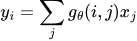
We will have to keep in mind that generating weights and applying the layer are separate operations, each contributing to resource consumption.
This recipe——could be a small neural network, a codebook, or a dynamical system; some architectures even use actual fractal functions.
We will start with trainable generators and gradually move on to random number generators with a fixed seed, local codes, and simple transformations in place of matrices. Along the way, we will touch on related ideas: KV cache compression and self-similar architectures. We will finish with an overview of shared blocks and repeated passes. First, we will examine the methods and budgets using their authors' results; some of these papers are recent 2026 preprints. At the end, we will see what came out of our selective checks on a CPU and a MacBook.
Contents
Three different budgets
As mentioned earlier, we need to consider several properties of a model that change when we replace its weights with a recipe. We will track changes in three quantities. Let us call them “budgets.”
Size on disk — the amount of storage the model occupies “at rest.” It consists mainly of the recipe: the generator and all the data needed to reconstruct the model's weights, such as latents, indices, scales, and any conventional weights left in place if the architecture replaces only some of the model's weights with a generator. We must keep in mind that a reduction in the number of trainable parameters does not necessarily mean an equivalent reduction in the size of the “model” file on disk. This budget, like the ones that follow, depends on the architecture of the particular model.
Working memory — the amount of memory (RAM or GPU memory) the model needs while running. What it includes depends on the implementation: we can reconstruct the entire matrix first, or generate its blocks piece by piece—obtain a block, multiply it by the corresponding part of the input, add the result to the output, and release the block. In the second case, we do not have to keep the entire matrix in memory at once, but we still need the generator itself, the current block, the layer's inputs and outputs, and intermediate activations. LLMs also need a KV cache: the stored attention keys and values for previous tokens.
Computational cost — the time the model spends preparing to run and performing the actual calculations. Sometimes weights can be reconstructed once at load time; sometimes reconstruction is part of every pass. We will therefore report preparation time and runtime separately. If the authors measure throughput—the number of requests or tokens processed per second—we will also state the conditions of that measurement. Reconstructing weights also requires computation; whether its cost can be hidden behind other operations depends on the implementation.
The design of the recipe determines which matrices it can describe. Different methods therefore have their own limitations. One of these is apparent from a simple count:  arbitrary weights of
 bits each give
 possible matrices. With a fixed decoder, a description consisting of
 numbers of
 bits each selects at most
 possibilities. If
 , it is impossible to describe every possible weight matrix without loss.
Now, finally, let us get to the most interesting part and look at specific generator architectures
A trainable generator: from hypernetworks to coordinates
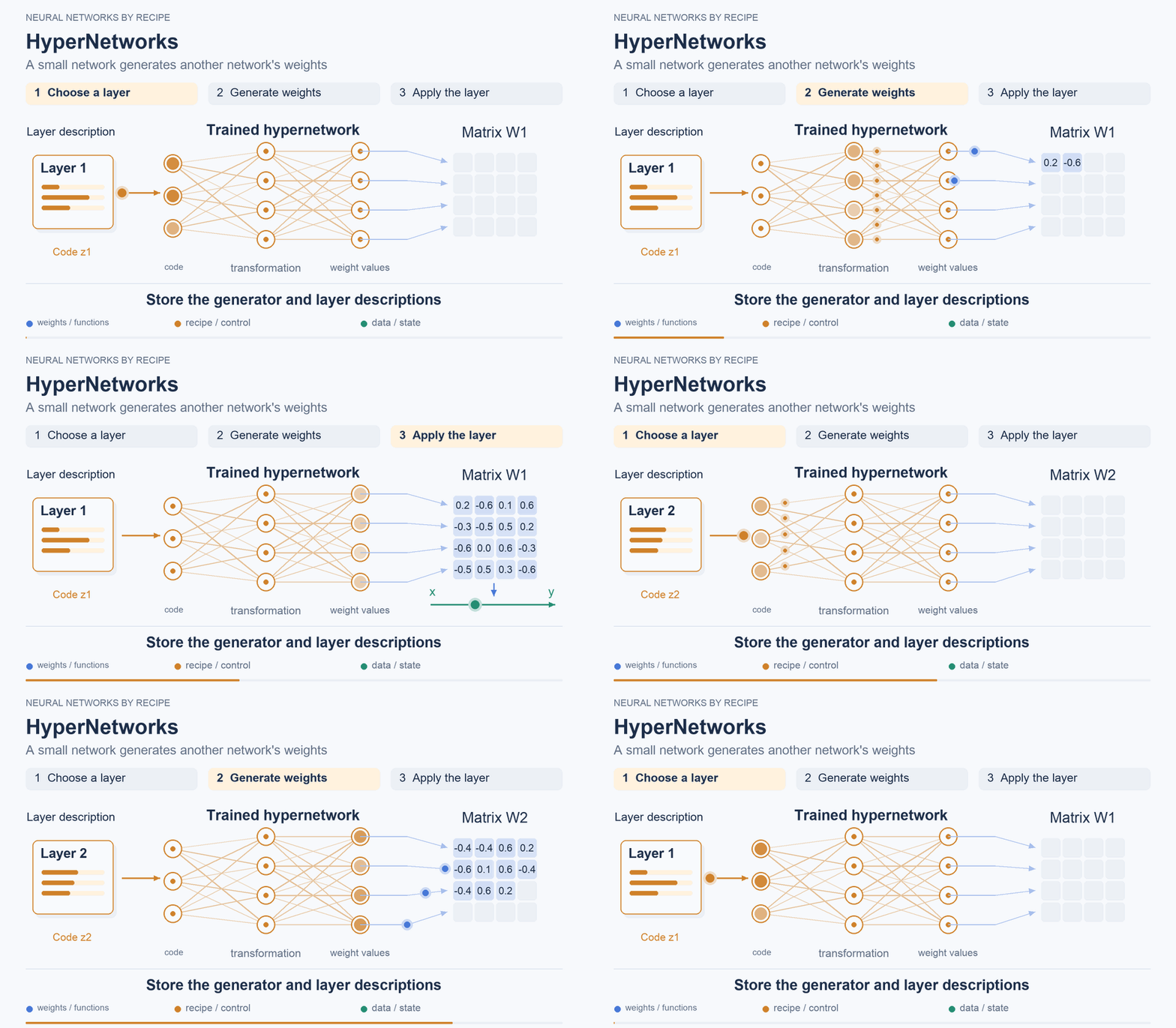
Probably the most obvious way to solve the problem of “generating some stuff that seems to have no pattern at first glance” is to use a neural network. This approach is called a hypernetwork: a network that generates another network's weights. In HyperNetworks, its input is a trainable description of a layer, and its output is the required filters. In the static version, the hypernetwork reconstructs dense convolution kernels. It is possible to expand them all in advance and then use an ordinary network. Reconstructing them layer by layer would avoid keeping all of them in memory at once—one possible implementation.
For Wide ResNet 40-2—a convolutional network with skip connections between layers and an increased number of channels—on CIFAR-10, a dataset of small color images in ten classes, the parameter count falls from 2.236 million to 0.148 million, but the classification error rises from 5.66% to 7.23%. In this experiment, the savings came at a cost in quality: there were fewer parameters, but the error increased.
budgets
Storage — the hypernetwork, layer descriptions, and remaining conventional parameters are stored instead of independent filters. File sizes are not reported; an estimate based on the parameter count in FP32 gives roughly 8.94 → 0.59 MB.
Memory — peak memory is not reported; dense kernels for 36 convolutional layers are reconstructed for execution. Expanding all of them brings the corresponding volume of weights back into memory.
Time — latency for this comparison is not reported; generation adds computation, but static weights can be reconstructed once before processing inputs. §3.1, §4.2, Table 2
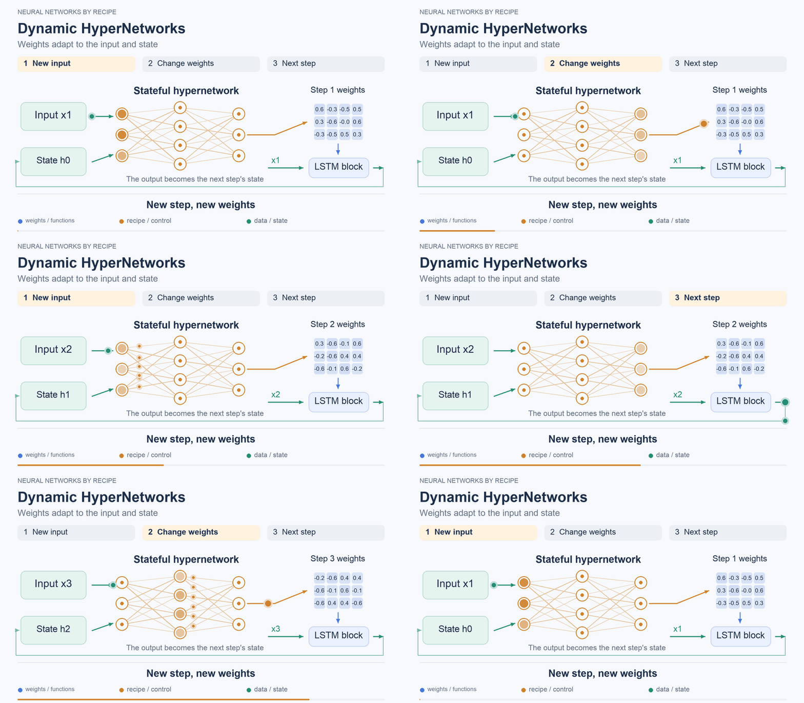
Dynamic hypernetworks are also worth mentioning. Their distinctive feature is that they change the weights they generate for the main network depending on its input and state. Their purpose, however, is usually somewhat different: greater expressiveness by adapting weights to the input and state. Such networks do not have to be smaller than the original network. The same paper tests this version on RNNs and LSTMs for sequences. For example, on Penn Treebank text, the network predicts the next character. A conventional LSTM has an error of 1.312 bits per character, versus 1.265 for HyperLSTM; here, lower is better.
budgets
Storage — file size is not reported; in this comparison, the parameter count rises from 4.25 million to 4.91 million because a hypernetwork is added to the main network.
Memory — a separate peak is not reported; the hypernetwork's states are also needed.
Time — there is no numerical latency comparison here; generation is invoked at every step. §3.2, Table 3
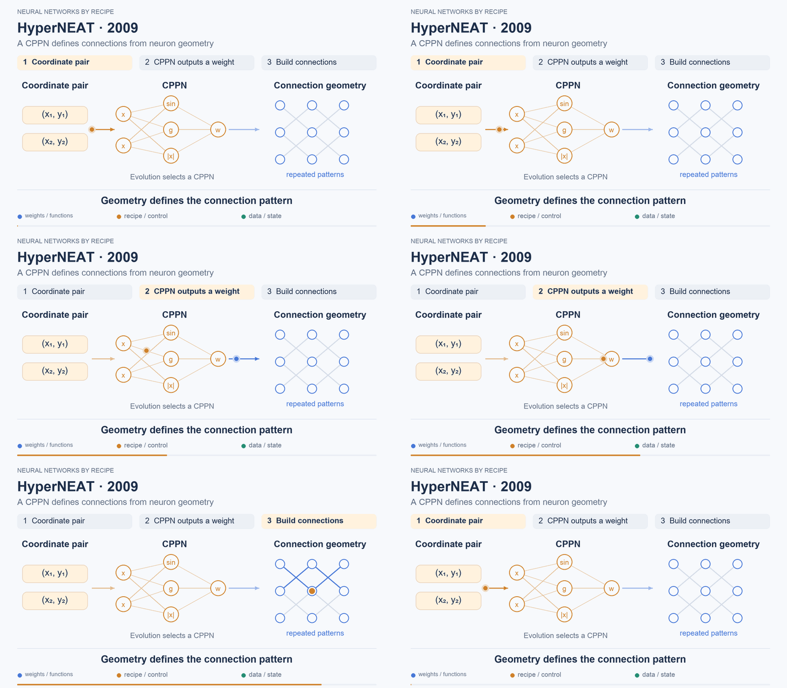
In the static hypernetwork above, the input was a layer description. We can go further and feed the generator the coordinates of two neurons, receiving the weight of the connection between them as output. A similar approach was tried as early as 2009 in HyperNEAT. Here, a small network defines a pattern of connections through the geometry of the neurons' positions. This makes it possible to describe symmetries and recurring motifs, and to search over the parameters of that description. But the task here is to evolve a suitable network, rather than pack the weights of an already trained one.
This was tested, for example, on a simple visual task: finding the center of a large square next to a small one. Quality was measured by the distance from the correct center. A generator found on an 11×11 grid was then used for 55×55 without a new evolutionary search. The resulting networks had an average of 8.3 million connections; the authors found no statistically significant decline in quality with this increase in resolution. §4–5, Figure 10
budgets
Storage — the generator and a description of the geometry can be stored instead of a list of all connections; file size is not reported.
Memory — peak memory is not reported; in the experiments, a network with generated connections is built first and then executed.
Time — generation and execution latency are not reported; the network is built before evaluating each candidate in the evolutionary search. §3, §5.1–5.3
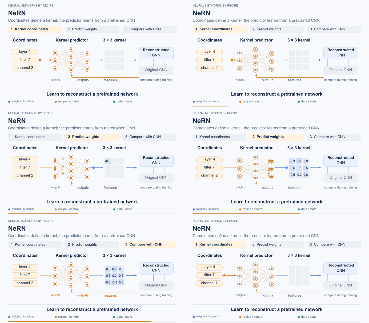
A coordinate-based representation can also be used for an already trained network. In NeRN, the coordinates are the layer, filter, and channel indices: a five-layer fully connected network takes them as input and outputs a convolution kernel. Here, there is already a trained CNN that the authors want to represent using a small predictor.
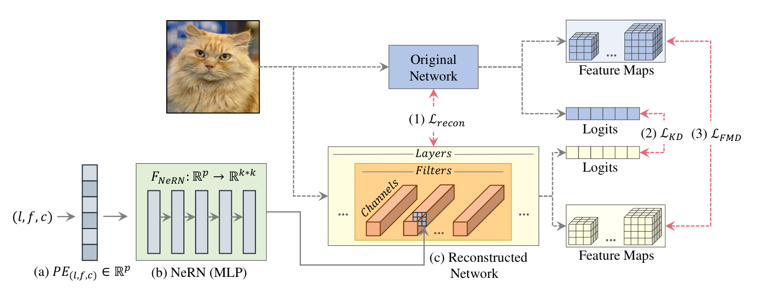
NeRN, Figure 1. On the left, coordinates are turned into weights; on the right, the reconstructed network is compared with the original in terms of weights, outputs, and intermediate features. p. 3
But matching the individual little numbers closely turned out to be insufficient: a small error in a weight can noticeably change the network's output. The predictor is therefore trained to reproduce not only the weights, but also the outputs and intermediate features of the original model. The authors also reorder the kernels so that neighboring coordinates describe more similar values; the inverse permutation must also be stored. §3
On ResNet20 and CIFAR-10, a 0.65 MB predictor reconstructs a network with an accuracy of 91.68 ± 0.06%, compared with the original 91.69%. Reducing it to 0.36 MB gives an accuracy of 90.39 ± 0.05%. Compactness here is controlled by the size of the generator itself, and at some point the effect on quality becomes noticeable. Table 1
budgets
Storage — the 0.65 MB predictor is compared with 1.03 MB of convolutional weights, rather than the complete package: this permutation also requires 0.04 MB of permutation maps and other conventional parameters.
Memory — the weights must be reconstructed for execution; peak memory for a streaming version has not been measured.
Time — the speed of the entire network including generation is not reported in this comparison. For now, this is a result for a CNN, rather than a language model. §3.1, Appendix C–D
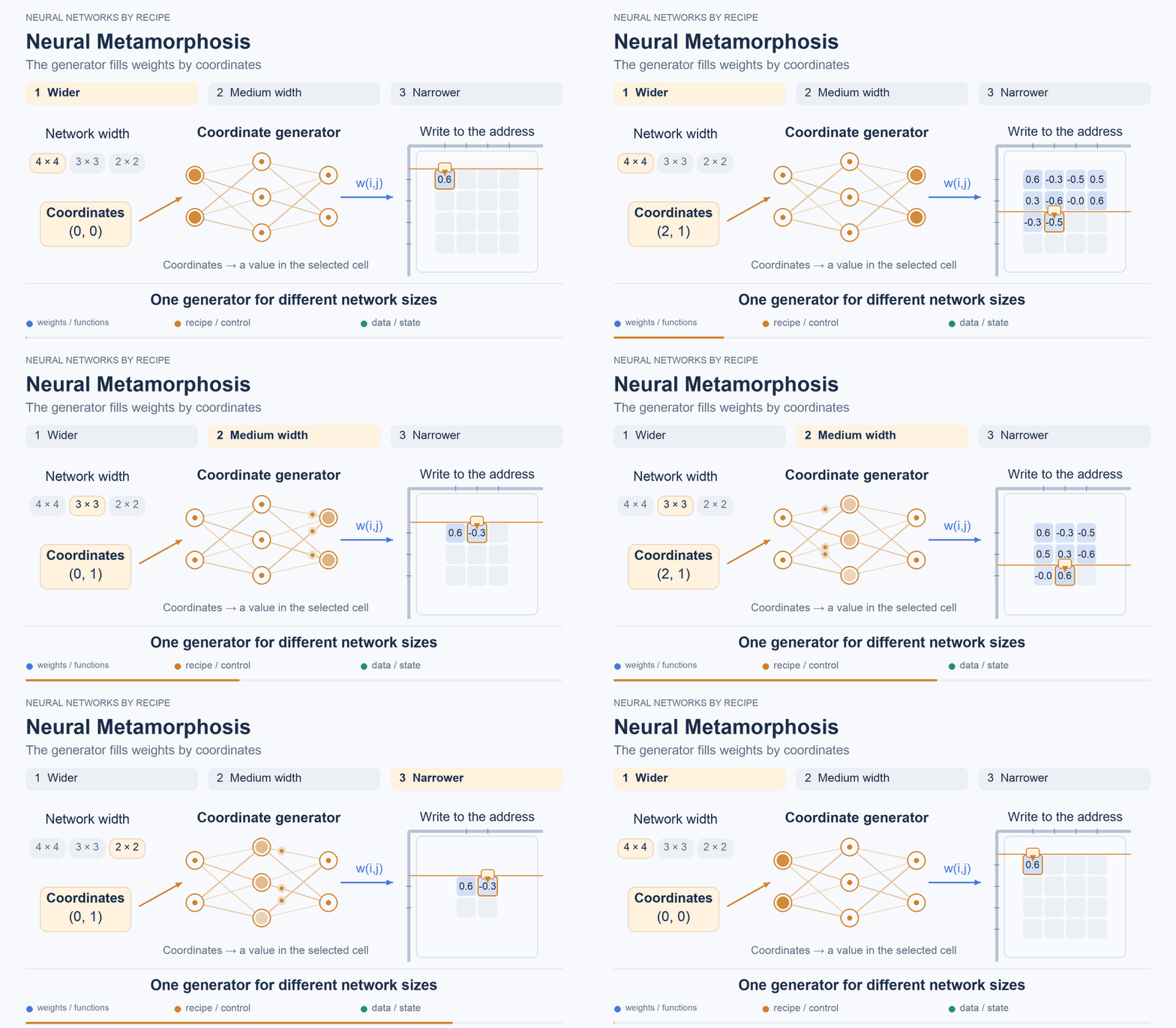
In Neural Metamorphosis, a coordinate-based generator is used for different network sizes: the authors generate weights and consistently reorder neurons, making the coordinate function easier to train. The weights for the chosen width are reconstructed before execution. The authors compare networks with the same width and the same cost for the main pass.
On CIFAR-10, its ResNet20—a 20-layer convolutional network with the same skip connections—achieves 91.76% at full width and 89.56% with a quarter of the channels. The authors describe this as 75% compression. However, if you look at the original paper, please note that “75% compression” means removing three quarters of the network's channels, rather than reducing the generator file by 75%.
budgets
Storage — file size is not reported; the table lists 0.20 million stored parameters for NeuMeta, versus 0.67 million for a set of separately trained networks of different widths. This is roughly 3.35 times fewer parameters for the entire set.
Memory — peak memory is not reported; the reconstructed weights for the chosen width and the activations are needed.
Time — latency including the generator is not reported; a narrower network requires fewer operations, but the coordinate-based representation itself does not make convolutions cheaper. §4.1, Table 2
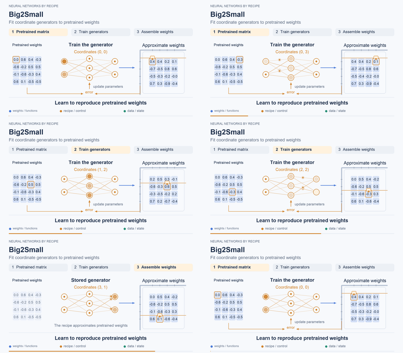
Another way to compress an already trained model is described in Big2Small: fit a coordinate-based network that approximates its weights. The generators reconstruct the weights, which are then loaded into the original architecture for a conventional pass. Besides ResNet, the method has been tested on the Swin vision transformer and a convolutional U-Net for image segmentation.
On ImageNet—a large image dataset, used here for classification into a thousand classes—the accuracy of ResNet18, an 18-layer convolutional network, changes from 71.47% to 71.24%.
budgets
Storage — 44.6 → 7.6 MB for ResNet18, or 5.9×. Two sources of savings are at work here: the generator and six-bit quantization. Without quantization, in FP32, the recipe takes up 30.4 MB and achieves 1.5× compression. In the table, the 6/6 setting means six bits for both weights and activations.
Memory — peak RAM/VRAM is not reported; the compressed package on disk does not replace the reconstructed weights in working memory.
Time — in a separate test on ImageNet and an NVIDIA RTX PRO 6000, latency including weight reconstruction increased by about 30%. Figure 3, Table II, Inference Time
Seeds and latents: from kilobyte networks to LLM blocks and adapters
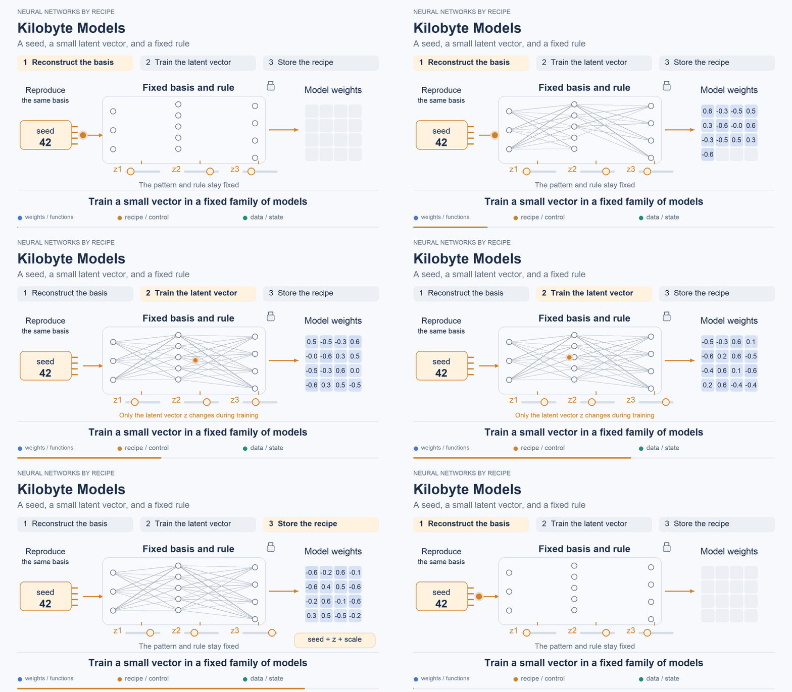
So far, our recipe has been another neural network, which also had to be stored. Can we make it even shorter? In Kilobyte Models, the authors keep a seed—a number that lets a pseudorandom number generator reproduce the same sequence—and a small trainable vector. This vector is called a latent: its values specify the model's position within a preselected family. The generator here is fixed: a random basis and initial weights are reconstructed from the seed, after which a predefined nonlinear formula is applied. There is no need to store a separate trained network for this.
It is easy to imagine a magical compression tool here: feed it any model and get a couple of kilobytes back. But compactness is built in during training—the authors train the model within a restricted family that the generator can reproduce. The seed itself contains no knowledge of the task; that knowledge must fit into the latent. In the setting shown below, the recipe consists of a seed, a scale, and 4,096 four-bit latent values; such a short representation is achieved through quantization-aware training.
The idea is tested on small convolutional networks, fully connected networks for tabular data, and a recurrent LSTM. For example, a CNN with 105,866 parameters achieves 98.60% accuracy on MNIST, a dataset of handwritten digits, versus 98.99% for the full FP32 model. On Fashion-MNIST, where the task is to distinguish items of clothing instead of digits, the result is 89.11% versus 91.06%. Still decent, but the recipe's limited capacity becomes more noticeable.
budgets
Storage — the compact description of the selected CNN takes up 2,060 bytes.
Memory — total peak memory including generation is not reported; after reconstruction, the network runs with conventional dense weights.
Time — there is no measurement including reconstruction; computation for the pass itself is not reduced. The authors state this explicitly: “do not compress inference compute.” Limitations
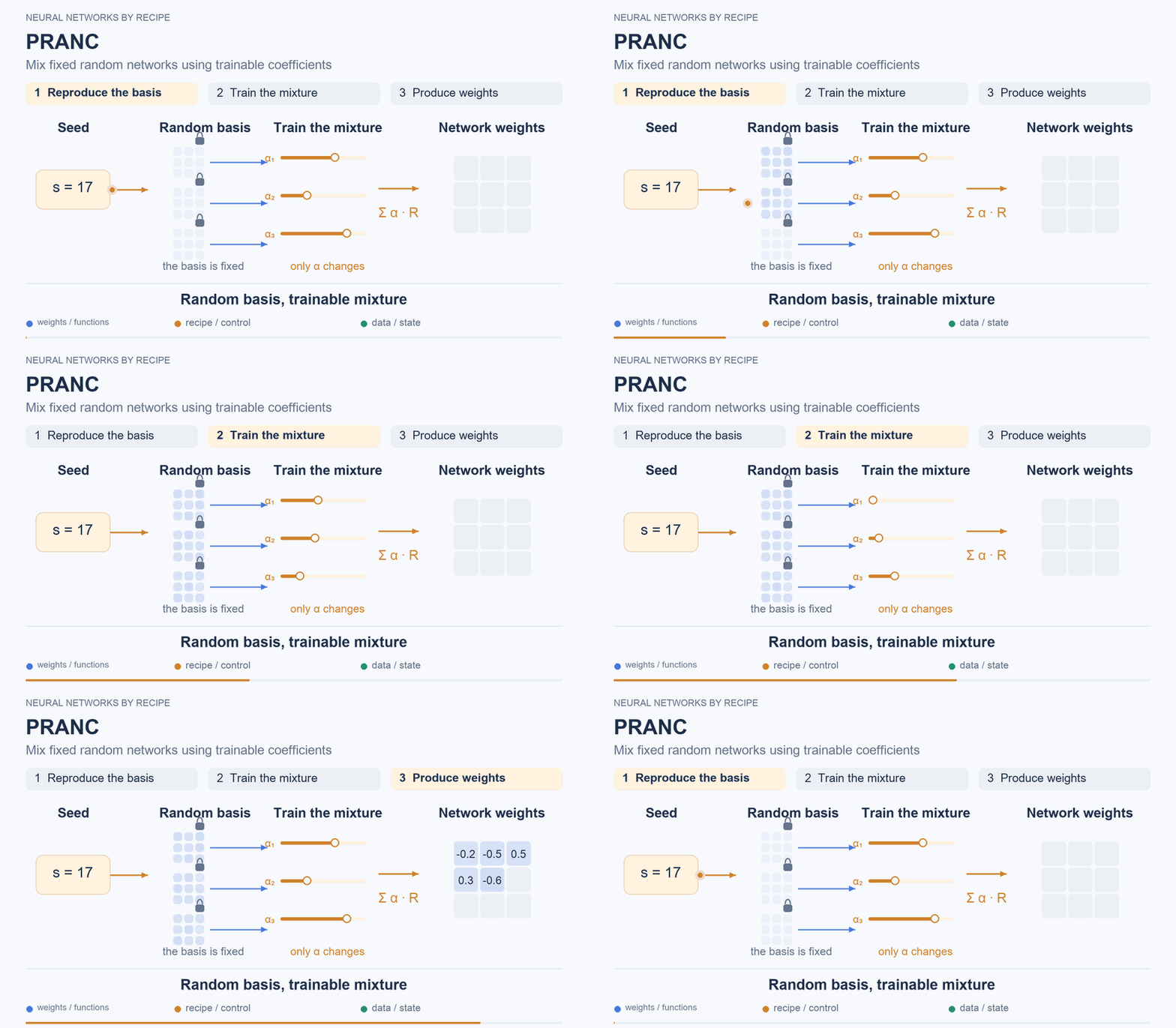
A random basis can also be used without a nonlinear generator. In PRANC, the weights are a linear combination of fixed random networks:
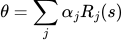 .
The seed reproduces the basis, while the coefficients  are trained. This is also training within a chosen family, rather than a way to losslessly store any existing network.
On ResNet18 and ImageNet-100, accuracy changes from 82.1% to 61.08%. The substantial reduction is clearly visible here, together with its cost. Table 4
budgets
Storage — instead of the original model's 11.23 million parameters, they store 100,000 coefficients, a seed, and 19,200 BatchNorm parameters; the size of the final file is not reported.
Memory — the authors describe reconstructing one filter at a time: obtain a filter, apply it, discard it. But peak memory for this execution mode has not been measured.
Time — latency with filter-by-filter reconstruction is not measured here. p. 4, Table 4
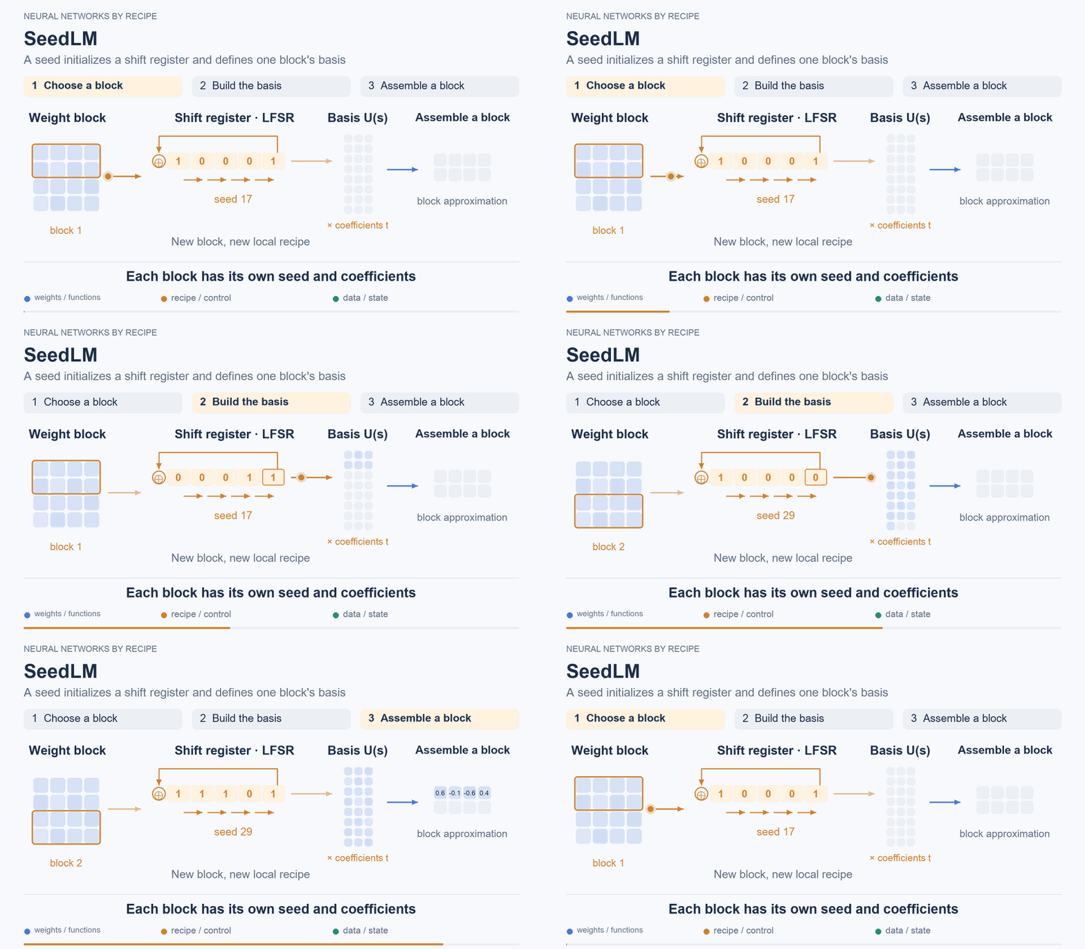
Meanwhile, SeedLM applies a similar idea to an already trained LLM. Here, though, the recipe describes a small block of weights, rather than the entire network at once. A seed and mixture coefficients are selected for each block. A simple pseudorandom sequence generator—an LFSR, a linear-feedback shift register—builds the matrix  from the seed, and the coefficients
 provide an approximation of the required block:
 .
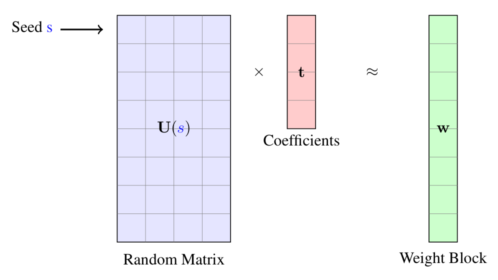
SeedLM, Figure 2. The matrix U(s) does not need to be stored, but a seed and coefficients are needed for each block. p. 3
The word “each” matters here: billions of weights do not fit into a single number. The savings arise because a block's local description is shorter than a list of its elements. The authors compress the model without calibration data or fine-tuning. For Llama 2-7B on WikiText-2 with a context length of 2048, perplexity—a token prediction metric for which lower is better—changes from 5.5 in FP16 to 5.7 with a four-bit representation and 6.6 with a three-bit one. But for Llama 3-70B, even the four-bit version gives 3.8 instead of 2.9: the same recipe does not imply the same loss in quality. Table 2
budgets
Storage — 3–4 bits per weight in the described format, including local seeds, coefficients, and scales; this figure does not describe the complete file.
Memory — the hardware implementation reconstructs weights for a matrix-vector operator; total peak memory for an LLM with its KV cache is not reported here.
Time — the FPGA operator achieves a 3.67–3.98× speedup. The compressed version uses 128 DSP blocks, compared with 32 for the FP16 version: fewer memory reads allow more compute units to be kept busy. This is a useful hardware result, but it is not yet the text generation speed of an entire LLM on an ordinary laptop. pp. 9–10
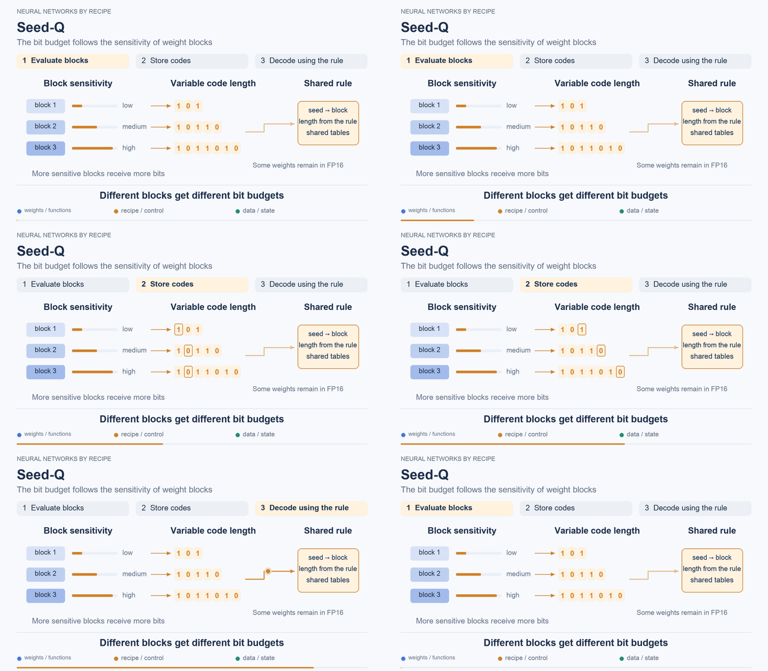
In Seed-Q, the same general principle remains, but more sensitive regions of the weights receive more bits. The decoder determines the number of bits for each block using a shared rule. There is no need to store a separate list for all blocks, although small shared tables and some weights in FP16 still remain.
For Llama 2-7B on WikiText-2 with a context length of 2048, the selected version achieves a perplexity of 5.85—the same as four-bit SeedLM in these authors' implementation. Table 1
budgets
Storage — the 3.77 bits per weight refer to the main code; auxiliary data, shared tables, and the remaining FP16 weights are counted separately. The size of the complete file is not reported.
Memory — total peak memory for the LLM is not reported; the authors estimate hardware costs through circuit synthesis.
Time — the speed of an entire LLM on a fabricated ASIC is not measured here. §4.2, Appendix A.7
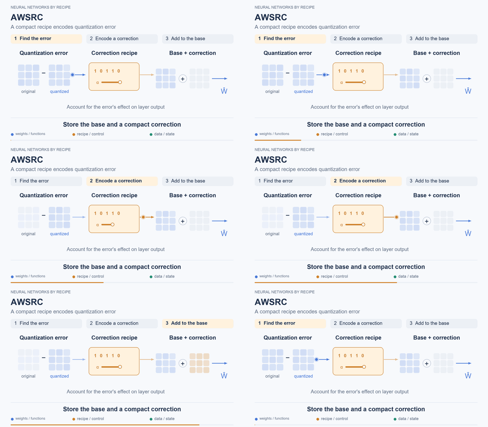
The same tool can be used to repair already compressed weights. In Activation-Weighted Seeded Residual Coding, or AWSRC, a seeded basis describes the error between the original matrix and its quantized version. The correction is chosen with the error's effect on the layer's output in mind.
In one experiment with Qwen2.5-3B-Instruct, WikiText-2 perplexity at a context length of 2048 changes from 9.834 after the initial compression to 7.075 with the correction, compared with 6.704 in BF16. Quality is evaluated after reconstructing the weights in BF16. The authors also test loading a self-contained package without the dense original. §4.2–4.3
budgets
Storage — the self-contained package takes up 2.60 GB; the correction itself adds 0.162 bits per weight of the replaced MLP matrices, rather than per parameter of the entire model. A small correction does not replace the model on its own: the compressed base and the other weights are also needed.
Memory — in this experiment, the weights are reconstructed in BF16; total peak memory is not reported.
Time — this experiment does not establish execution speed with the packed code. §4.2–4.3
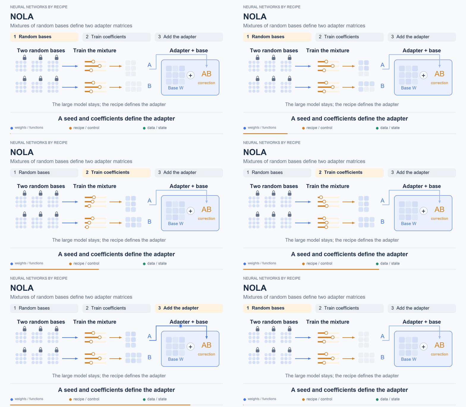
Finally, a recipe can describe only the correction learned during fine-tuning. In LoRA, this correction is specified by the product of two small matrices. In NOLA, these matrices themselves are represented as mixtures of random bases: a seed and learned coefficients are stored. The correction can be merged into the base in advance, yielding conventional dense weights with no extra operations during execution.
For eight-bit Llama 2-70B, MMLU accuracy with five examples in the prompt is 69.4% for NOLA, versus 69.5% for rank-1 LoRA. Table 5
budgets
Storage — the NOLA adapter contains 0.57 million parameters, compared with 12.94 million for LoRA; file sizes are not reported. The main 70B model is not included in this comparison of adapter sizes.
Memory — in a separate GPT-2 L training experiment on an RTX 6000 Ada, memory remains around 33.4 GB for both approaches, so it does not fall by the same proportion. This is training memory, rather than peak inference memory.
Time — once the correction is merged into the base, there are no extra operations; no separate latency measurement is reported in this comparison. Table 2, Table 5, §3.1
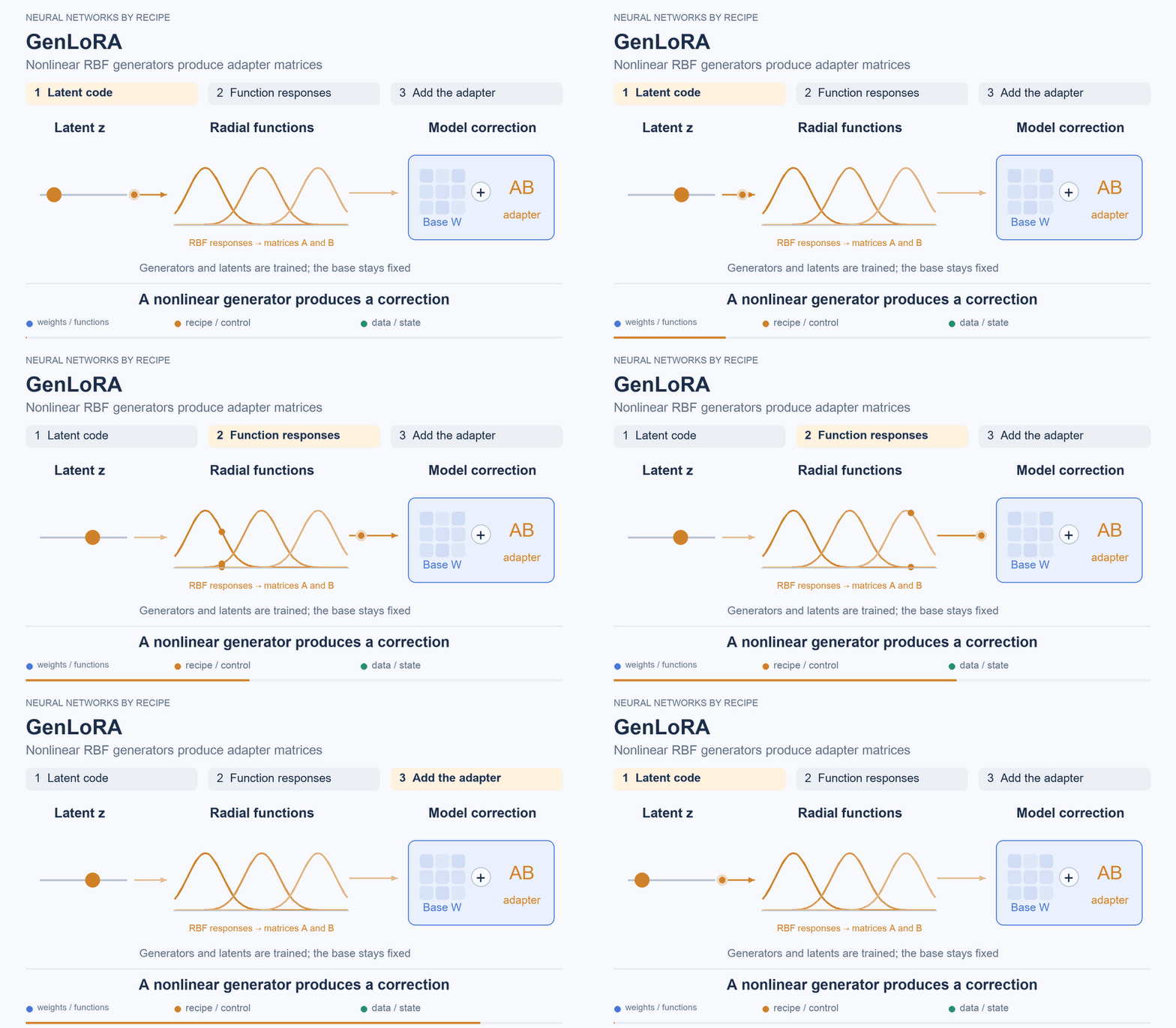
In GenLoRA, lightweight nonlinear generators with radial basis functions (RBFs) are used instead of a fixed random mixture. They generate the same small correction matrices from latents. As with NOLA, the correction can be merged into the dense base.
On Llama 3-8B after training on Math10K, average accuracy across six mathematics tasks is 70.17%, compared with 67.28% for LoRA. Table 1
budgets
Storage — the adapter in this comparison contains 0.98 million parameters, compared with 4.72 million for LoRA; the size of the complete package including the main model is not reported.
Memory — in a separate training experiment on coding tasks using an RTX A6000, peak GPU memory falls only from 31,724 to 30,460 MB. This is training memory for the entire system, rather than the adapter's size or peak inference memory.
Time — in the same experiment, training takes roughly the same amount of time: 11.6 → 11.7 hours. Inference latency is not measured here; once the correction is merged, the dense base runs. Table 1, Appendix G.4, Table 9
Codebooks, trajectories, and blockwise computation
Now let us look at another way to approximate an already trained large model. A single short latent may be too restrictive for it, but nothing prevents us from storing many small codes and a shared way to decode them. It is a bit like replacing repeated words in a text with their dictionary indices—except that here, the reconstructed pieces of weights may differ slightly from the originals.
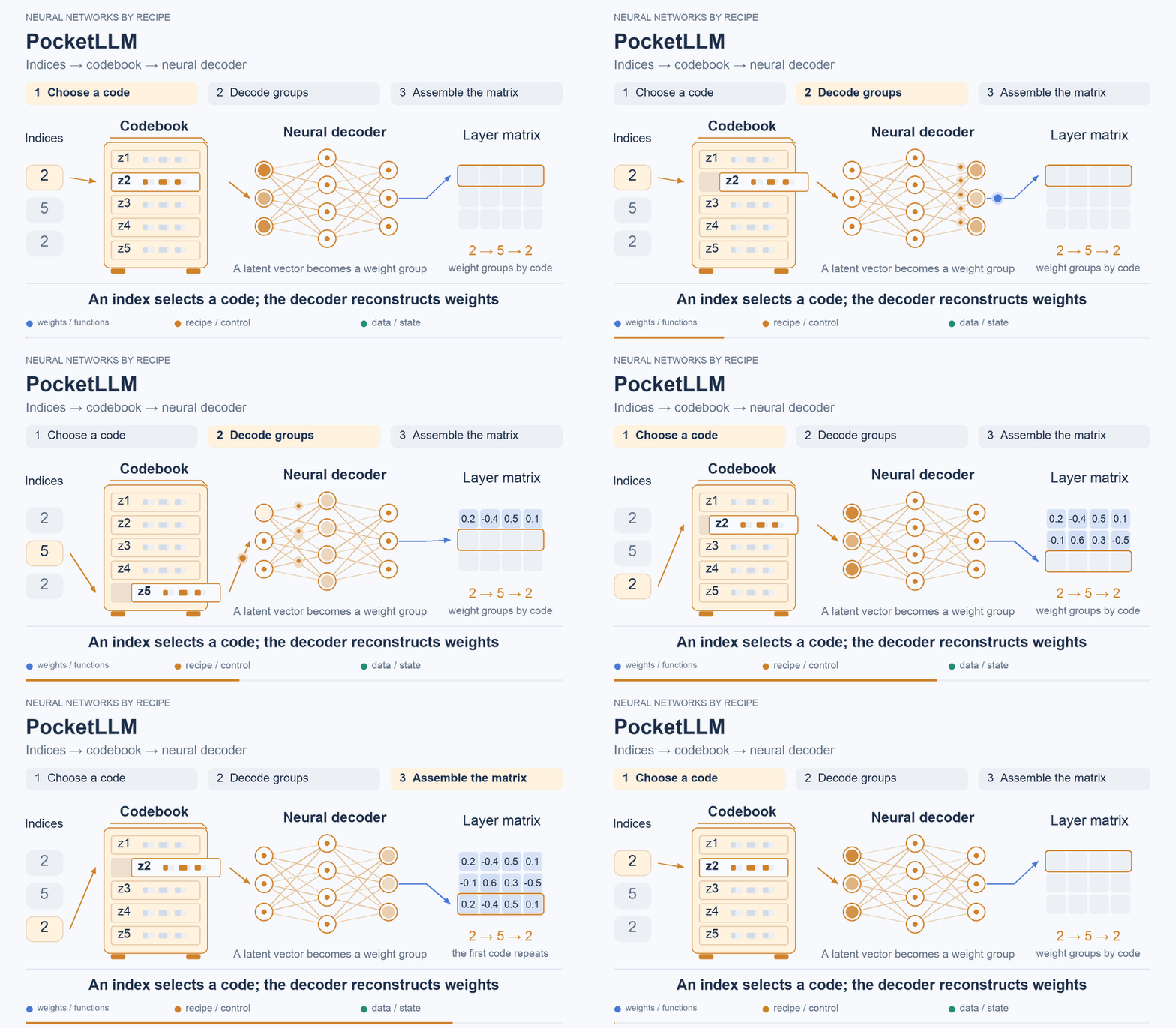
In PocketLLM, this dictionary is called a codebook. It is a table of latent vectors: an index selects a row, and a small neural decoder turns it into a group of weights. The full recipe includes the indices, codebook, and decoder. After loading, the decoded groups are assembled back into layer matrices.
The method is tested on the Llama2-7B and Qwen3-14B language transformers. For Llama2-7B, at 2.98 bits per compressed weight, average accuracy across five tasks after fine-tuning is 64.07%, versus the original 64.29%. Without fine-tuning, it is 59.53%; at 1.60 bits, even with fine-tuning, it is 55.45%. In other words, the small file is achieved here not only by choosing a code, but also through additional training.
budgets
Storage — 2.98 bits per compressed weight in the reported setting; the complete file size is not reported. The claimed “about 10×” is calculated relative to FP32 and the compressed weights being counted; it is not the reduction factor for the entire file, and certainly not a promise to compress an already four-bit model another tenfold.
Memory — peak memory is not reported; reconstructed weights, activations, and a KV cache are needed.
Time — latency including decoding is not reported; reconstruction adds operations, but the authors do not report measurements of their effect on startup time. Algorithm 1, Compression Ratio Analysis
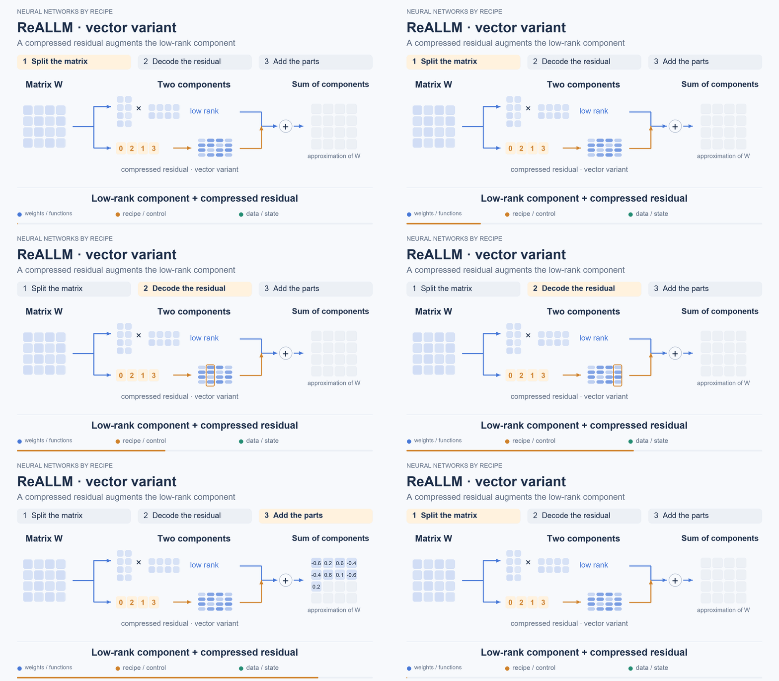
This representation of weights can be combined with a conventional low-rank component. In ReALLM, the matrix is represented as the sum of this component and a compressed residual. Both vector quantization and the HNeRV neural decoder are available for the residual. A result from a particular table therefore cannot automatically be attributed solely to the neural version.
A two-bit version is tested on Llama 2-7B with a context length of 2048. The rank of the low-rank component is 64, and the vector quantization dimension is  : values in the latent representation are grouped in fours. Without fine-tuning, WikiText-2 perplexity is 40.85; after the full fine-tuning cycle, it is 6.69; for FP16, it is 5.47. The small code here works together with additional training. Tables 1–2
budgets
Storage — besides the compressed residual, the low-rank components, decoder data, scales, and other weights are needed; the complete file size for this comparison is not reported.
Memory — total peak inference memory is not reported.
Time — preparing Llama 2-7B, including compression and fine-tuning, takes about 90 hours on an A40; this is preparation time, rather than response generation time. The execution speed of the entire model is not reported in this comparison. §4
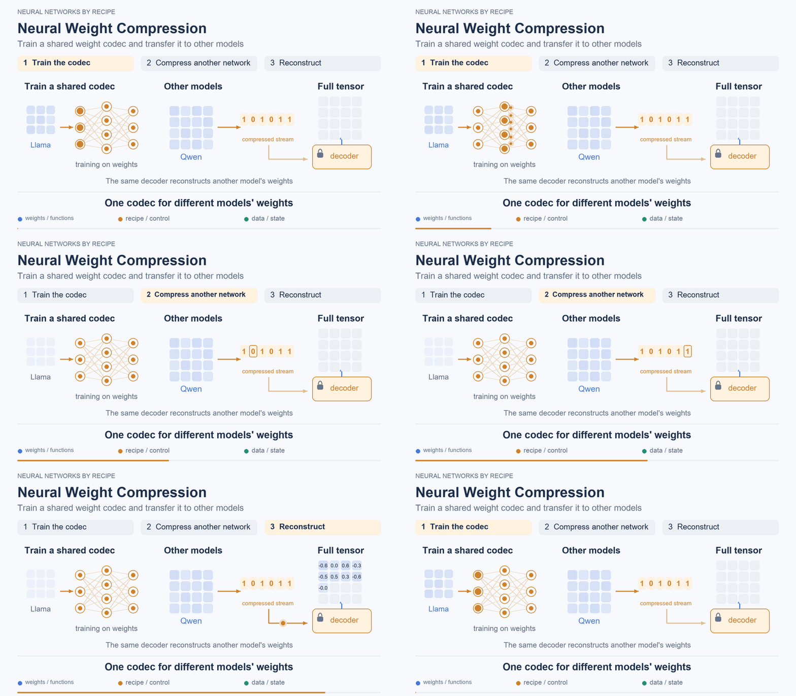
In Neural Weight Compression, the authors go further: they train a shared codec on a collection of weights and then apply it to other models. A probabilistic model for entropy coding is trained alongside the decoder, giving frequent values shorter descriptions.
The codec, trained on Llama 3-8B, is tested on Qwen among other models. For Qwen3-8B in the selected setting, the average result across four reasoning tests is 69.0%, versus 70.0% for the 16-bit base. This result includes additional fine-tuning during compression: the as-yet-uncompressed layers within each block are adjusted to account for the errors of the already compressed layers. Table 1
budgets
Storage — 3.94 bits per weight in the reported setting; the size of the complete package with the shared decoder is not reported.
Memory — the implementation is studied at the level of individual tensors and reconstructs them in full; total peak memory for the model is not reported.
Time — the authors leave fused tile-wise decoding to future work; this comparison does not establish faster response generation. Table 1, Limitations
A shared decoder does not necessarily have to be a neural network, though. In Hyper-Compression, the authors use the trajectory of a dynamical system—an irrational winding on a torus. Stripped of the geometric name, the recipe looks fairly simple. A numerical code is selected for each group of weights. Multiplying it by specified coefficients and taking the fractional parts of the results lets us approximately reconstruct that group. Each group has its own finite-length codes, scales, and auxiliary parameters.
In the mathematical model, the trajectory can come arbitrarily close to the desired points. But the index of a suitable location on it also has to be stored, and a short code may not be enough for a more accurate approximation. There is no fractal function in this mechanism. To avoid waiting for the entire model to be unpacked, the authors propose reconstructing subsequent layers in parallel with the execution of earlier ones. The decoding cost remains, but some of it can be hidden behind computation.
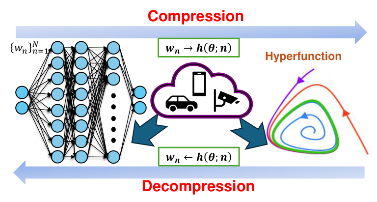
Original Figure 1 from Hyper-Compression: parameters are replaced with a description, then reconstructed. The practical algorithm stores many local codes. p. 2
The method is tested both on convolutional image models and on LLMs in the LLaMA and Qwen families. For LLaMA2-7B, average accuracy across eight tasks changes from 65.88% to 64.89%: a loss of 0.99 percentage points. WikiText-2 perplexity rises from 5.47 to 5.82. In the same table, GPTQ int4 gives a perplexity of 5.69. In this comparison, GPTQ is both more compact and has lower WikiText-2 perplexity. Tables 5–6 The average scores for PocketLLM and Hyper-Compression cannot be compared directly: they use different sets of tasks.
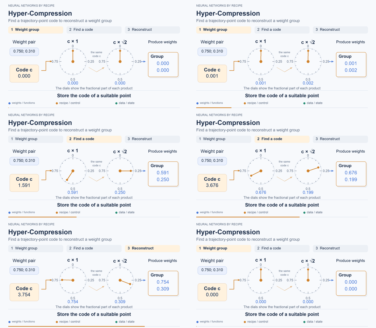
budgets
Storage — LLaMA2-7B: 12.50 → 4.80 GB, or 2.60×; GPTQ int4 achieves 3.46× in the same table.
Memory — peak memory for this LLaMA2 comparison is not reported; the recipe and expanded layers that are already in use or have been prepared are needed.
Time — LLaMA2 latency is not reported. For U-Net at batch=1, the results are 4.35 → 4.43 seconds on an RTX 4060 and 1.50 → 2.06 seconds on an A40. These are measurements for another model; they cannot be used to calculate LLM latency. §4, Table 15
The next logical question is: why create the full layer matrix in the first place if we are about to multiply it by the input? In Birkhoff / HyperLinear, decoding a block of weights is fused with matrix multiplication. Reconstruct a block, use it, move on to the next. This is a practical example of the option we discussed in the section on working memory.
The implementation uses CUDA/Triton; porting such an operator to a low-powered CPU is a separate engineering task. The method has been tested on GPUs and models in the SAM family for segmentation—identifying objects in an image. For example, for SAM-B on COCO with box prompts, segmentation mAP changes from 37.0% to 36.8%—a loss of 0.2 percentage points. This paper does not provide results for LLMs. Table VI
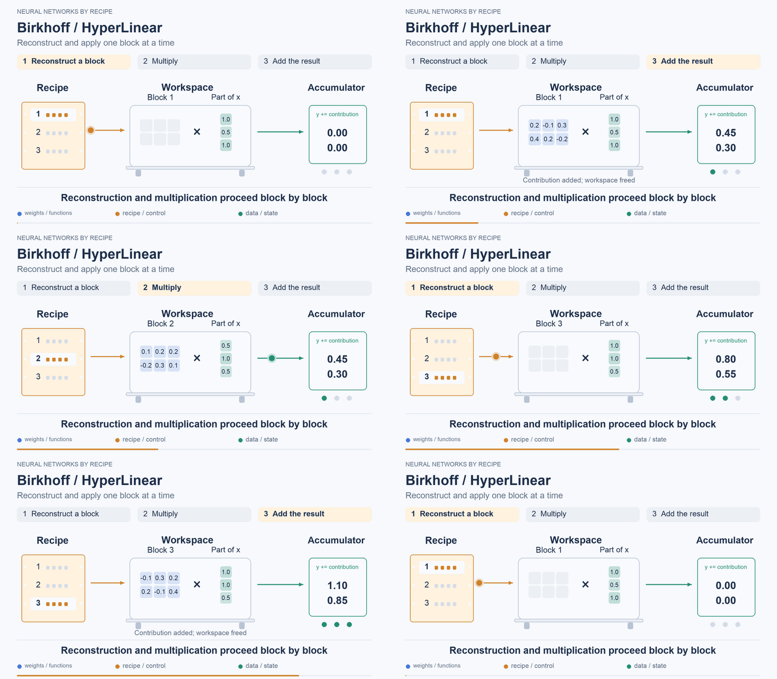
budgets
Storage — compression for SAM-B in Table VI is 4.31×; in the abstract, the authors report 5.17× for SAM2-B. When stored, the indices are tightly packed: each is allocated the required number of bits. In terms of compression ratio, the method does not yet outperform INT6.
Memory — total peak VRAM is not reported; the full matrix of the replaced linear layer is never created, but the recipe, working blocks, activations, and other weights remain. In HyperLinearV1, there is one uint16 index for every pair of weights: about eight bits per original weight even before auxiliary data. This is the working index matrix, rather than its packed representation on disk.
Time — in Table V, all six tested compressed SAM models run more slowly than the originals; fusing decoding with multiplication reduces overhead compared with performing these operations separately. Table V, index packing, HyperLinearV1 implementation
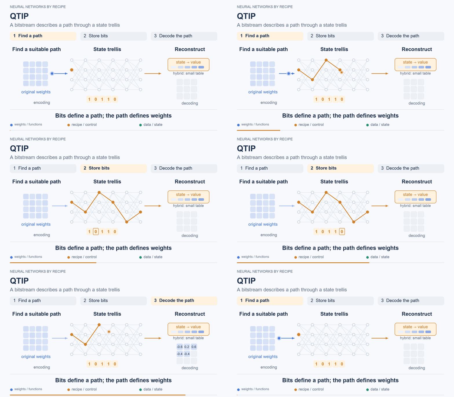
There is also a paper, however, that evaluates a compact code by measuring the speed of an entire LLM. In QTIP, instead of independently choosing a codebook row, the authors use a code with a lattice of states—a trellis. Its state shifts as bits are read, and the sequence of states defines the reconstructed weights. A long sequence is encoded at once here, allowing its structure to be taken into account without creating an enormous table of every possible combination.
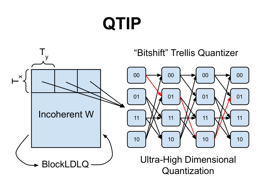
QTIP, left panel of Figure 1. A block of weights is encoded by a path through the trellis; a weight's value is specified by the decoder of the selected state. p. 2
The value corresponding to a state does not necessarily have to be stored in a table. QTIP has variants where it is computed using a few simple instructions, and a hybrid version where a formula selects a row from a small table. Before encoding, the authors also change the basis of the weights using a randomized Hadamard transform. The pseudorandom decoder does not discover the weights on its own: the required sequence of states is selected during compression. §3
The purely computational 3INST variant on Llama 2-7B, WikiText-2, and a context length of 4096 gives a perplexity of 5.17 with a four-bit representation, versus 5.12 for FP16. At two bits, it rises to 6.82. There is no fine-tuning in this experiment. Speed is measured separately for the hybrid decoder. These are two variants of the recipe; combining the quality of the first with the speed of the second would be misleading. Table 3
budgets
Storage — a bitstream, auxiliary parameters, and a 2 KiB table for the hybrid; the 2 or 4 bits in the mode name do not describe the entire file.
Memory — decoding is fused with multiplication, but this does not establish the overall peak with the KV cache.
Time — two-bit Llama 2-7B with the hybrid decoder produces 188 tokens/s versus 55.9 for FP16 on an RTX 6000 Ada, batch 1. This measures text generation by the whole model, rather than just the speed of a single operator. Whether the same effect holds on a low-powered CPU or Metal still needs to be checked. Table 4, §4.2
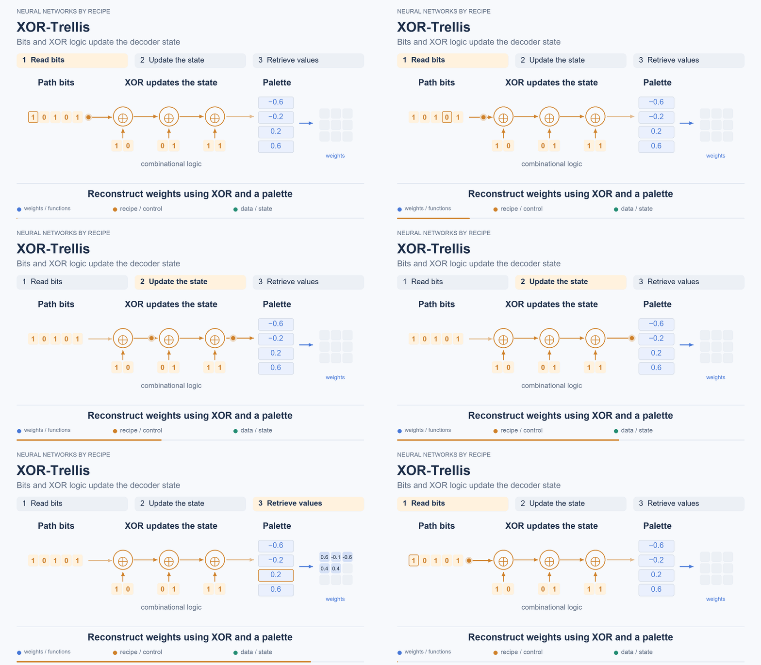
The recent XOR-Trellis continues this line of work: a weight value is reconstructed using simple XOR operations and a small palette, with no Hadamard transform required at runtime. Code selection takes into account how the error affects the layer.
On Llama 3.1-8B, WikiText-2, and a context length of 4096, the authors obtain a perplexity of 8.00 versus 5.84 for BF16, without fine-tuning but with calibration. Table 1
budgets
Storage — about 2.25 effective bits per weight, including scales; the size of the complete model file is not reported.
Memory — the overall peak for the LLM is not reported; there is an estimate of the hardware decoder's area, but that is a different quantity.
Time — this estimate does not yet establish the generation speed of the whole LLM on such a device. §5
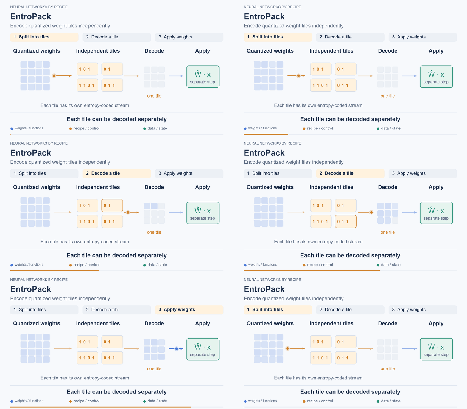
Another option is to store the coordinates of quantized weights and pack them using entropy coding: frequent values get short codes. In EntroPack the stream is divided into small blocks, or tiles. Each can be unpacked independently, without reading the preceding ones. The GPU operator reads the code and immediately reconstructs the numerical weights, while the subsequent multiplication remains a separate operation.
For the Z-Image-Turbo image generator, the error in the weights themselves is lower than for the NF4 variant used for comparison: 7.18% versus 9.41%. Weight error, however, is not the same as image quality. Table 1
budgets
Storage — 4.02 bits per weight in the selected linear layers, including metadata, versus 4.50 for NF4. These are compressed layers, rather than the full package with the text encoder.
Memory — the overall peak for the model is not reported for this comparison; weights are reconstructed in tiles, and multiplication is performed separately.
Time — one denoising step on an NVIDIA H20 takes 544.7 ms versus 505.7 ms for BF16. This timing excludes the first step, prompt processing, and the final image output. For long input-text processing, the cost of unpacking is easier to hide behind computation; this result does not establish ordinary fast LLM decoding. Table 1, Appendix A.1/A.5
A formula instead of a matrix: spectrum and simple factors
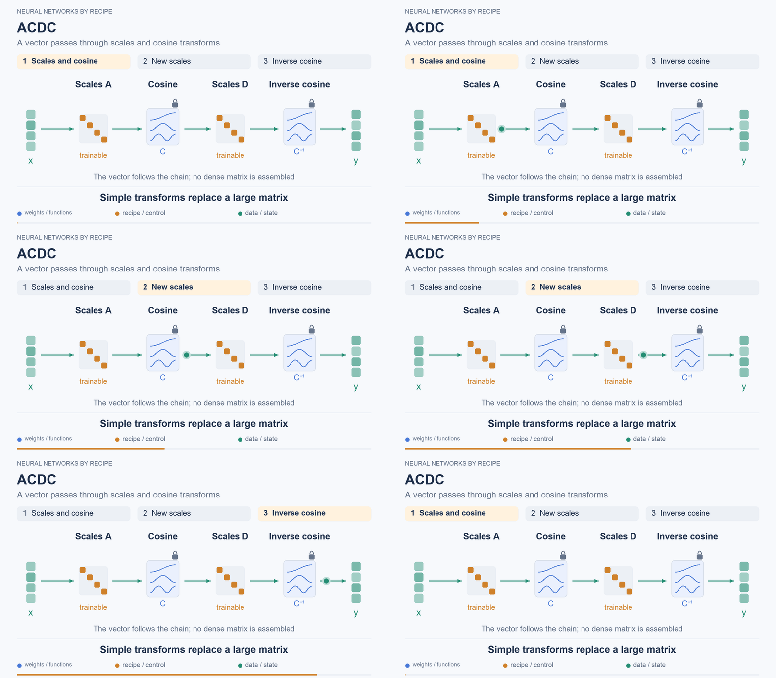
In the previous recipes, we reconstructed weights, sometimes directly during multiplication. But multiplication itself can be specified through a few simple transforms. In ACDC a single large matrix is replaced with a sequence of operations: scale the vector's elements individually, transform them into cosine coefficients, scale them again, and transform them back. The scales are learned, while the cosine transform is fixed. Writing the input vector as a row gives
 ,
where  and
 are trainable diagonal matrices,
 is the cosine transform, and is the size of the input vector. One such module requires
 parameters and
 operations; several modules can be placed in sequence. There is no need to build a dense matrix for execution.
In CaffeNet on ImageNet, the authors replace two fully connected layers. Top-1 error increases by 0.67 percentage points. Table 1
budgets
Storage — the parameter count of the whole model changes from 58.7 to 9.7 million; the size of the complete file is not reported. This is a reduction in the parameter count of a CNN.
Memory — there is no need to build the dense matrix of the replaced layer, but the overall peak for the model is not reported.
Time — the authors measure the speed of a single layer on a Titan X, for both the forward and backward passes. This is a separate operator test; it cannot establish the response time of the whole model or justify promising a sixfold speedup from the reduction in parameters. §5, Figure 2
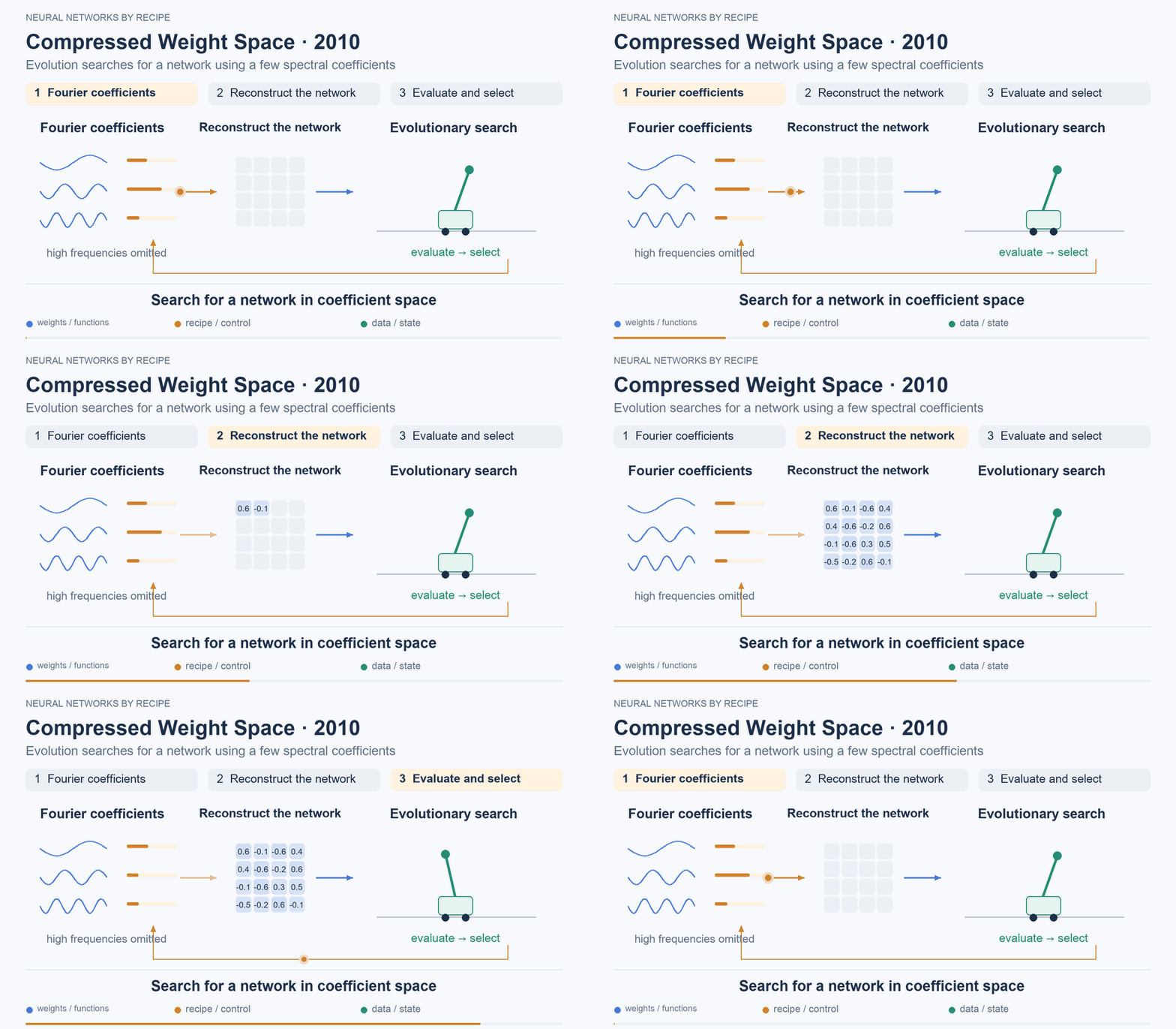
In ACDC, the cosine transform is part of the computation of the layer itself. In Evolving neural networks in compressed weight space, a 2010 paper, spectral coefficients serve as a compact representation of weights: evolutionary search operates on Fourier coefficients, which are then used to reconstruct matrices. High frequencies are discarded to reduce the search space. The authors study control tasks, including pole balancing and controlling an octopus arm. Here, they search for a suitable network in a compact representation, rather than compressing an existing network.
In the octopus-arm simulation, a recipe of 40 coefficients specifies a network with 728 weights. The mean score of the best controllers found is 0.38 versus 0.17 for direct search over all weights, across 20 runs. This score accounts for movement time and distance to the target; higher is better here. §3.3, Table 3
budgets
Storage — in this experiment, 40 DCT coefficients and a description of the architecture suffice instead of 728 weights; the file size is not reported.
Memory — the peak is not reported; the network's matrices are reconstructed from the coefficients before a candidate is evaluated.
Time — there is no measurement of the latency of the final network; the number of candidate evaluations in the paper characterizes the efficiency of evolutionary search. §2.1–2.2, Tables 1–3
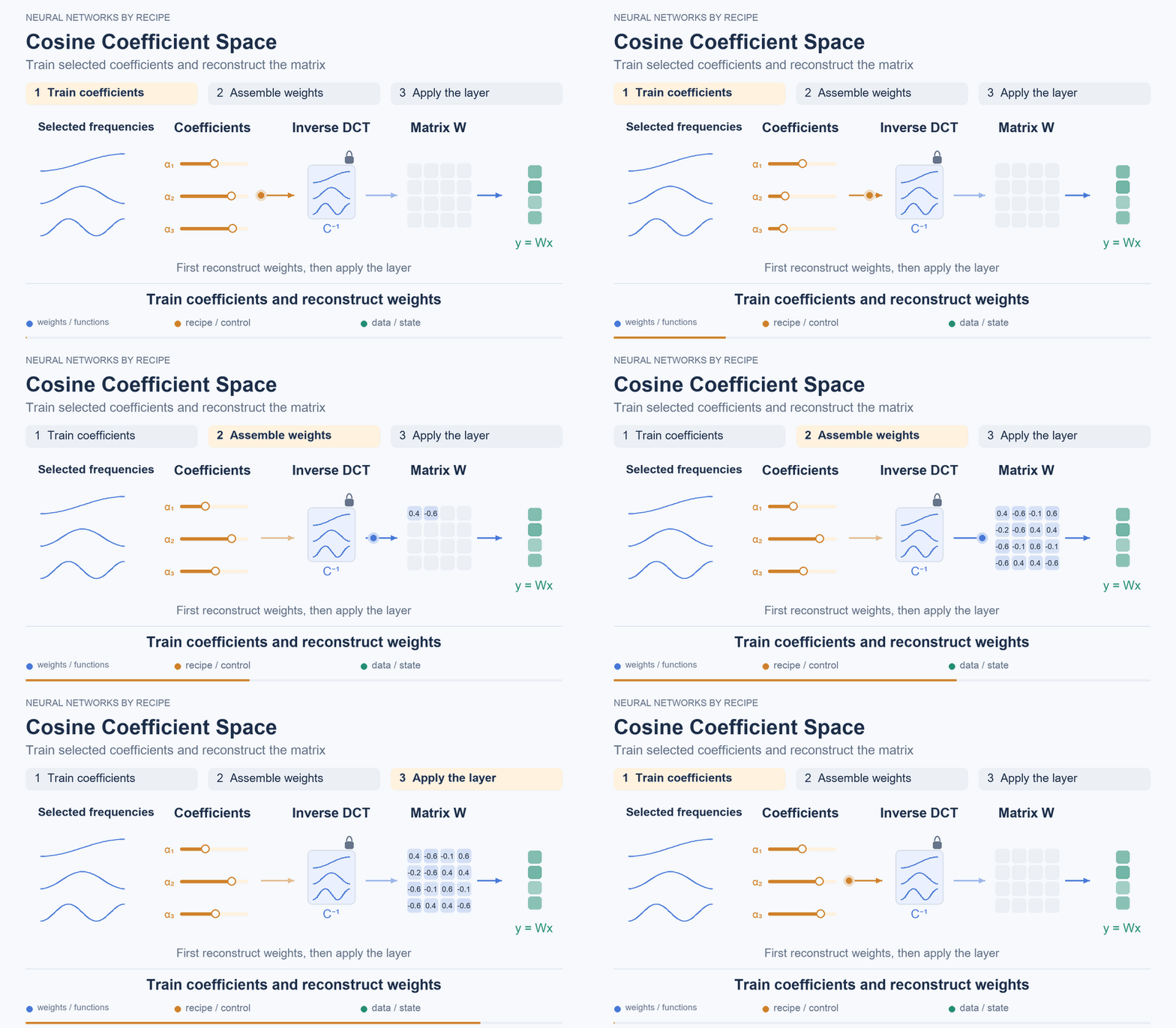
In the preprint Training Transformers in Cosine Coefficient Space this idea is tested in training a small language transformer. The attention and FFN matrices are specified by selected DCT coefficients, the coefficients of the cosine transform. Before each pass, weights are reconstructed using the inverse transform.
For a four-layer character-level model on tinyShakespeare, validation loss changes from 1.580 to 1.604. This is a small experiment with a single seed; it cannot establish equal quality for large LLMs. Table 1
budgets
Storage — the number of trainable parameters decreases from 818 048 to 424 832; the size of the final file is not reported.
Memory — a dense matrix is still created in the main experiment; the overall peak is not reported.
Time — the authors discuss a prototype on Metal, but leave measuring fused reconstruction and multiplication during training to future work. The speed of the whole model with this execution approach is not established here. Table 1, p. 5
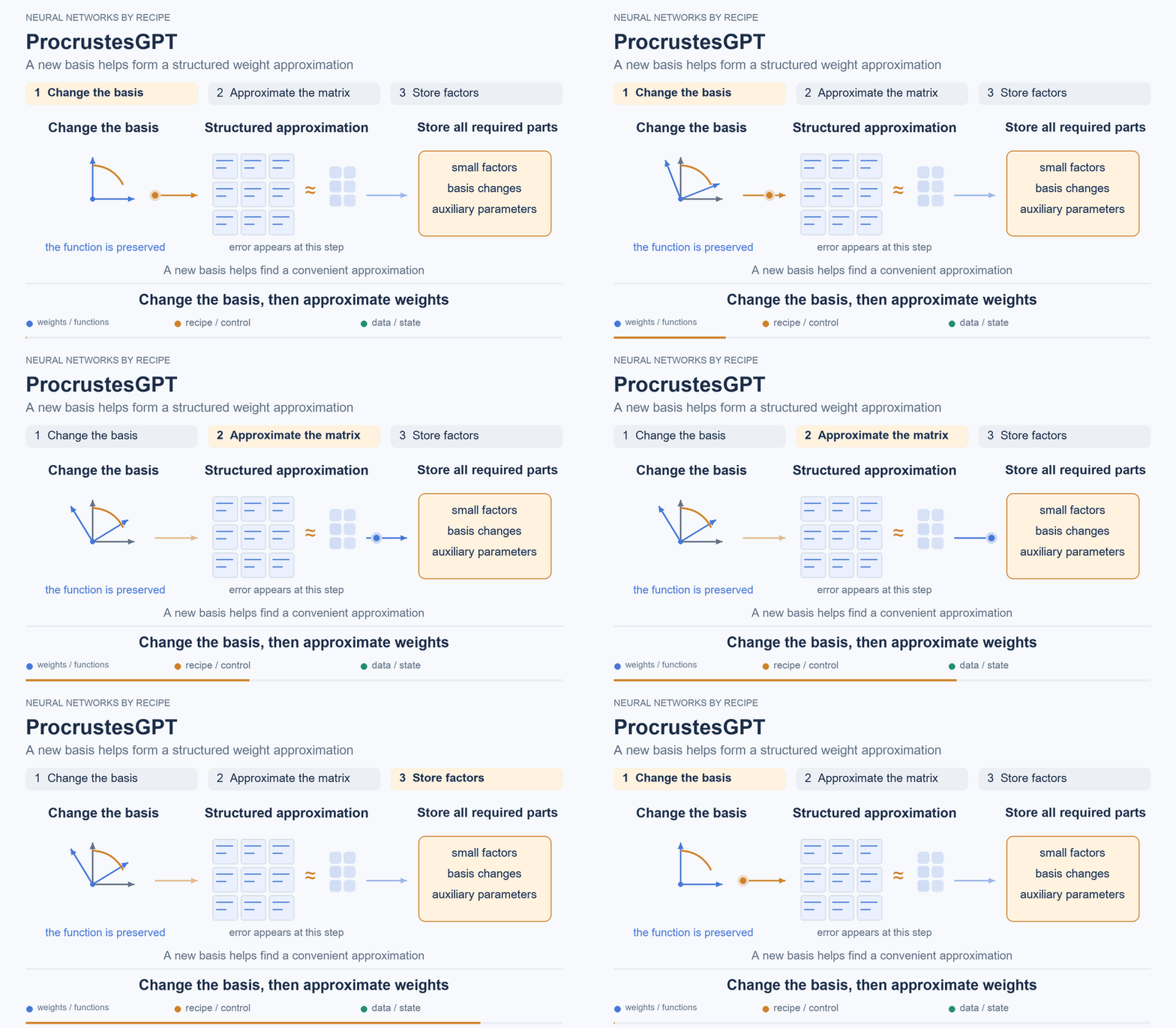
An existing LLM, however, need not immediately reveal a convenient structure in its weights. In ProcrustesGPT the authors first rewrite the weights in a different basis. To do so, they select coordinated orthogonal transforms that preserve the behavior of the original model. They then approximate the weights with structured matrices. One option is a sum of Kronecker products, where a large matrix is assembled from small factors.
On Llama 2-7B, WikiText-2 perplexity rises from 5.47 to 8.19. Calibration data is used, but there is no fine-tuning to recover quality. Preserving behavior under a change of basis does not make the subsequent approximation lossless. Table 3
budgets
Storage — this variant reduces the parameter count of the whole model by 25.09%; the transforms themselves are also part of the recipe. The size of the complete file is not reported.
Memory — the overall peak is not reported for this comparison.
Time — generation speed is not measured here; reducing the parameter count alone is no substitute for that measurement. Table 3, §5.4, §6
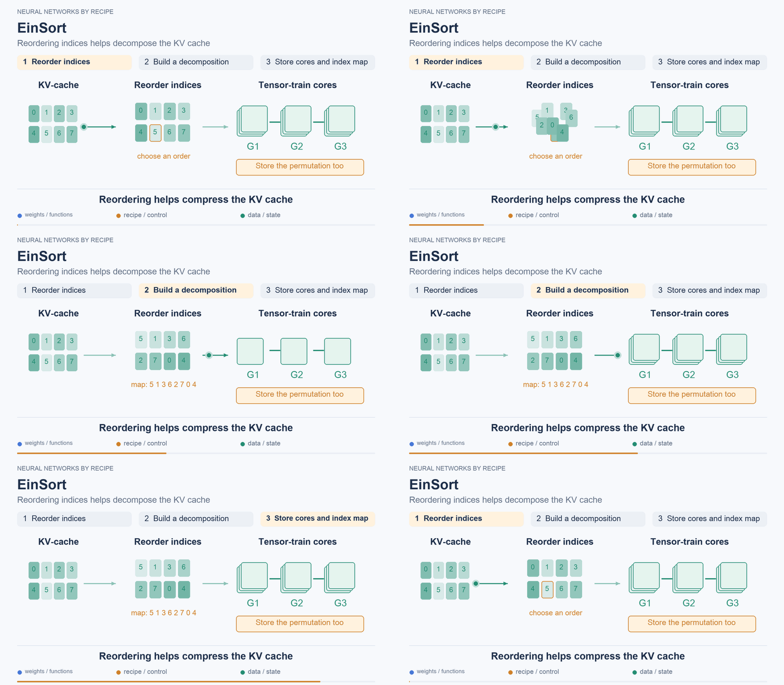
Now let's take a brief detour from weights to the KV cache. This is a related problem: it involves compactly representing intermediate data rather than model parameters. It is relevant to our question about a hypothetical kettle, which needs memory for both weights and context. In EinSort permuting indices helps uncover a structure suitable for tensor decomposition. But the ordering also has to be stored, and a full permutation map can wipe out all the savings; the authors use shared permutations for groups of elements.
In the main execution experiment with Qwen3-0.6B, 64 tokens are processed first, the cache is compressed, and then up to 64 new tokens are generated. In the mode the authors call “Compression 90%,” the tensor train variant, a chain of small tensors, gives a perplexity of 27.04 versus 47.38 for the SVD variant in the same experiment. These numbers compare two variants of the compressed cache; they do not reveal how much quality was lost relative to the original cache. Tables 2–3
budgets
Storage — reducing the weights file is not considered in this experiment: it is the cache that is compressed.
Memory — “90%” here denotes the cache decomposition mode. The full cost, including the permutation and sign bits, is not reported; nor is the overall peak for the model.
Time — speed on an A40 is only 61.9% of that of the model without cache decomposition. The better cache representation comes at the cost of extra work here; this experiment does not show a speedup of the whole model. §3, Tables 2–3
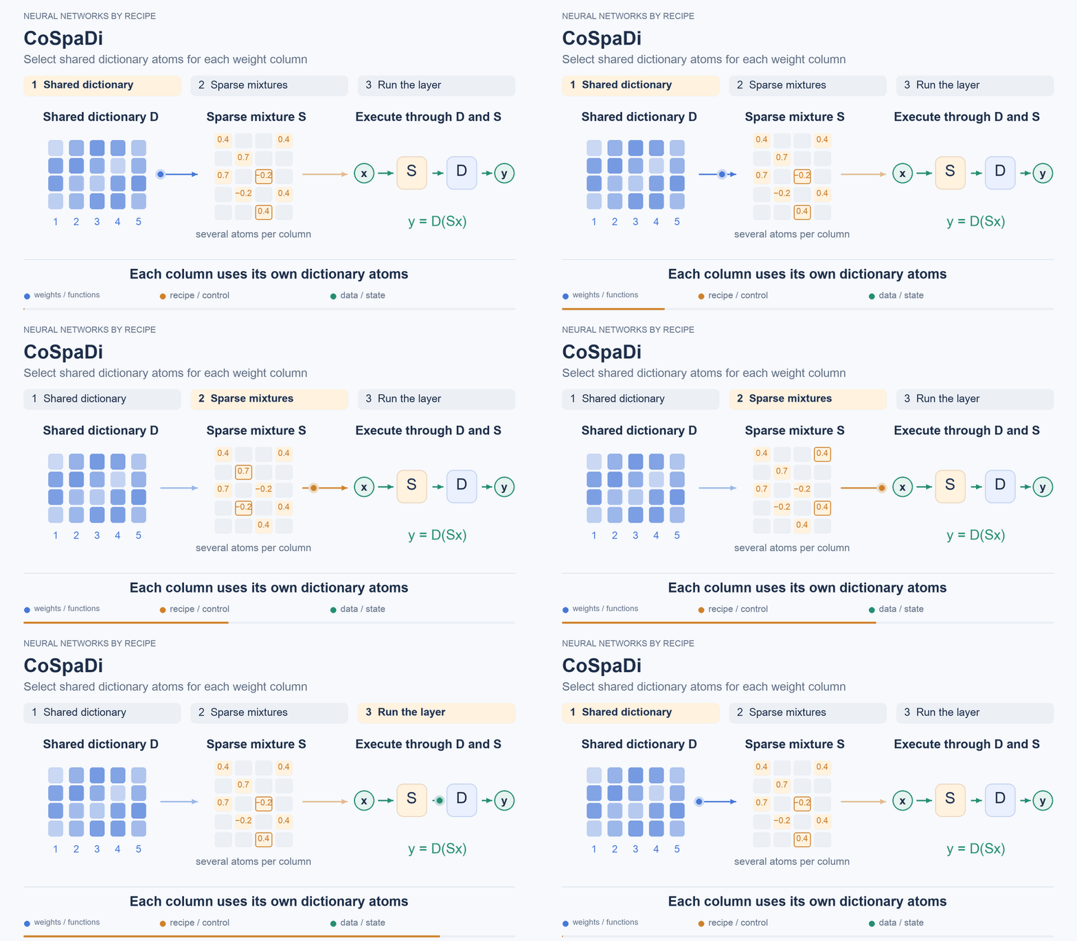
Let's return to weights. In CoSpaDi different columns of a matrix can use different sets of elements from a shared dictionary. A dense dictionary and sparse coefficients are stored: they specify which elements to take and with which multipliers. Selection takes into account activations on calibration data, and the layer is executed directly through the dictionary and coefficients.
To test execution, the authors separately compress only the up and gate expansion projections of Llama 3-8B. In the mode with a 40% reduction in their representation, average accuracy across eight tasks changes from 70.4% to 61.9%. The SVD variant used for comparison is faster but has worse quality. Table 6
budgets
Storage — the 40% reduction applies to the representation of the selected projections, which includes the dictionary, coefficient values, and masks; the size of the complete model file is not reported.
Memory — the overall peak with the KV cache is not reported; the layer is executed through the dictionary and sparse coefficients.
Time — average synchronous generation speed on an RTX 3090 is 48 tokens/s versus 44 for the dense model, for prompts ranging from 1 to 256 tokens. This measures a whole LLM with selected replacements, rather than a speedup of any layer or any compression mode. Table 6, Appendix A.11/A.15
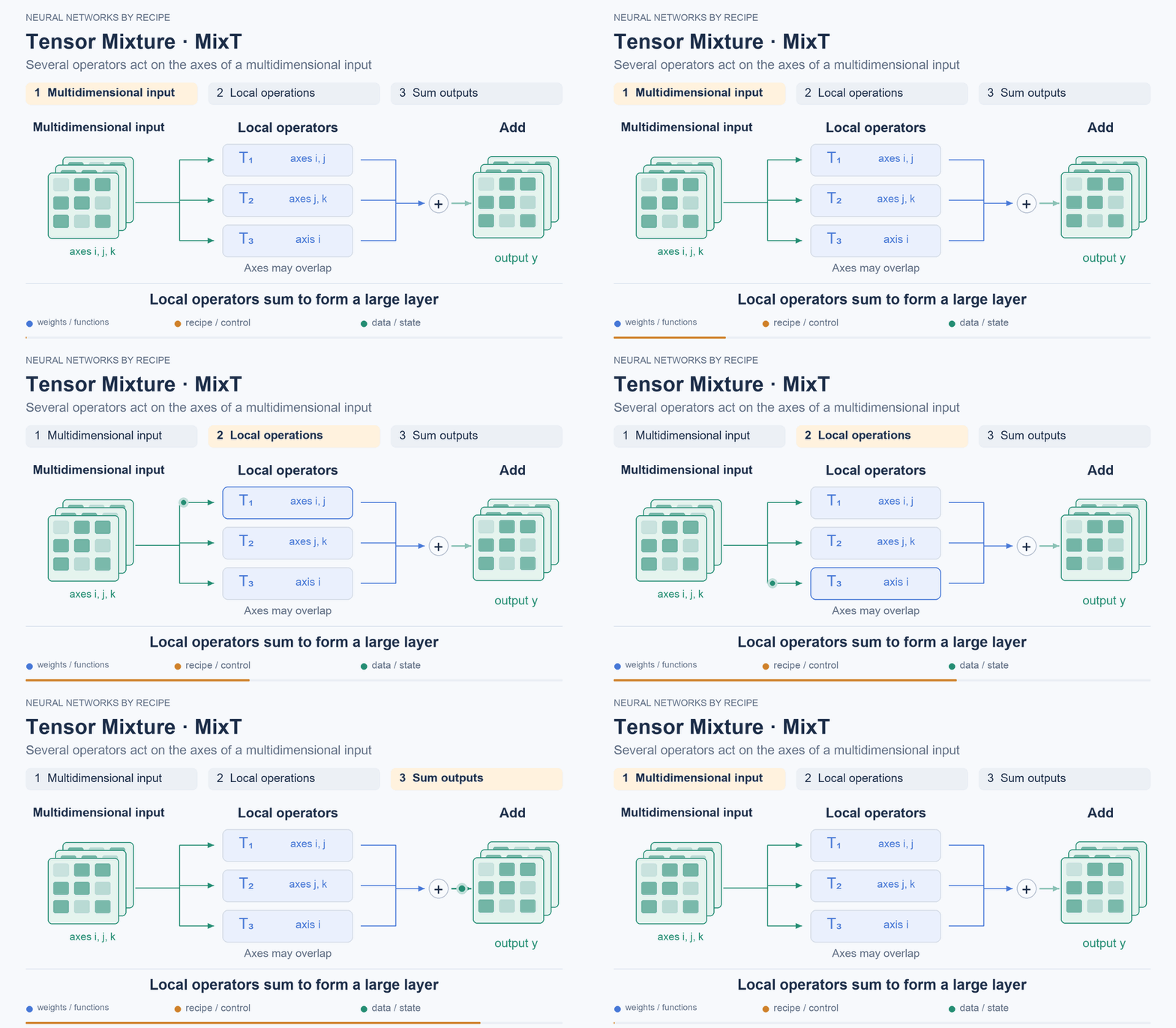
In CoSpaDi, matrix columns are specified through a shared dictionary and sparse coefficients. Another option is to decompose the action of the layer itself into several small transformations of the input. This is how Tensor Mixture, or MixT works: instead of one large multiplication, several small ones are performed and their results are added. To do so, the input is represented as a multidimensional array. Each part operates on several of its axes, leaving the others unchanged; different parts may operate on the same axes. These parts are called local tensor operators. This allows the layer to be executed without assembling a dense matrix. The number of local parts and the number of replaced transformer blocks can be varied; after replacement, they are fine-tuned.
In one Llama 2-7B variant, 17 blocks are replaced. With four local parts, MMLU accuracy after fine-tuning is 43.56% versus 46.38%. Quality falls sharply as more blocks are replaced. §IV, Table I
budgets
Storage — the parameter count of the whole model changes from 6.74 to 3.58 billion; the storage costs in the paper are estimates, rather than measurements of a final file.
Memory — the measured peak during inference changes from 12.61 to 6.79 GiB. The complete measurement conditions are placed in a separate appendix that is absent from the available text.
Time — FLOP estimates are given rather than measurements of token generation speed; the layer can be executed without assembling a dense matrix. §IV, Table I
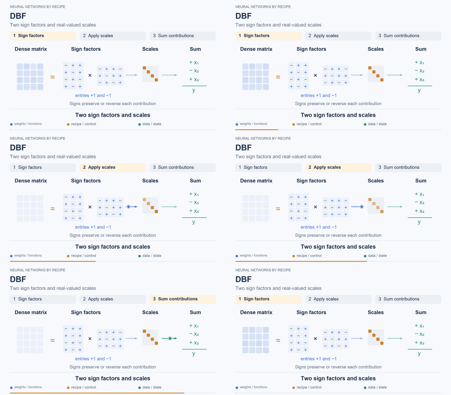
In MixT, the results of small transformations are added. Another option is to approximate a matrix with a product of simple factors. In Double Binary Factorization, or DBF, there are two such factors: sign matrices with real-valued scales. The sign matrices contain only −1 and +1. The intermediate dimension controls compactness and accuracy, while multiplication by signs allows some ordinary multiplications to be replaced with additions.
On Llama 3-8B, with an average budget of 2.3 bits per original weight, the variant with additional fine-tuning of matrix scales and signs (PV) gives a WikiText-2 perplexity of 6.86 versus 5.54 for the dense model. Fine-tuning is already required to prepare the base DBF, and PV adds another stage. Table 2, §3.4, §4.1
budgets
Storage — the average DBF budget in these experiments is 2.3 bits per original weight; the size of the final file containing all parameters is not reported.
Memory — the overall peak for the model is not reported.
Time — in a separate generation measurement, the whole Llama 3-8B produces 121 tokens/s versus 60 for FP16 on an RTX 4090. The conditions are batch 1, 128 tokens from an empty prompt, and a compiled graph; the DBF budget is the same 2.3 bits. This is a real speedup of full decoding on a GPU. Table 5, §4.4
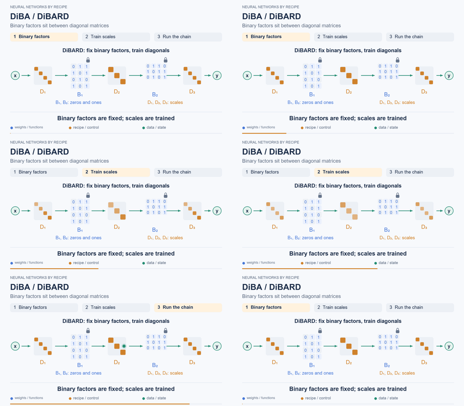
In DiBA the two factors contain only zeros and ones. Trainable scales, three diagonal matrices, sit between them and on either side. The formula looks like this:
 ,
where  and
 are binary matrices. The DiBARD variant fixes the binary parts and fine-tunes only the diagonals.
For example, this replaces 48 attention projections in an Audio Spectrogram Transformer that classifies speech commands. Accuracy is 76.84% after replacement, 97.81% after fine-tuning the diagonals, and 98.37% for the original model. The model's other weights are left in their ordinary form. Table 3
budgets
Storage — size is calculated from theoretical bit packing, rather than from a final file.
Memory — runtime memory use is not measured; an implementation using ordinary dense operations may store binary factors as floating-point numbers and take up more space than the estimate.
Time — unlike DBF, inference speed is not measured here. §6, Appendix C
Fractals on edges and in network topology
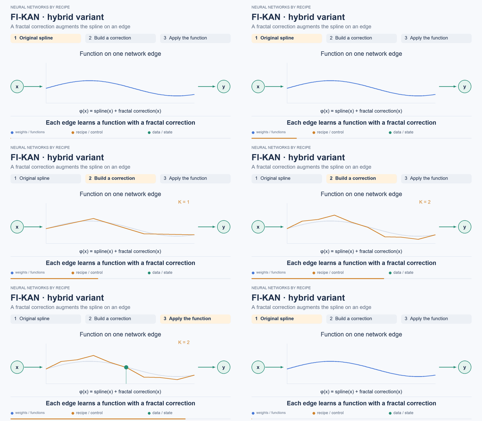
In FI-KAN a fractal appears: it participates in the transformation of the input itself. In an ordinary KAN, the edges between nodes carry trainable functions; here, those functions are built using fractal interpolation, repeated contractive transformations. In the pure variant, this replaces splines, which are functions made of joined polynomial pieces. In the hybrid, the splines remain, and a fractal correction is added to them.
These networks are studied on function approximation: given an input number or coordinates, the model must approximate the desired value. In a comparable evaluation, the hybrid achieves lower error on three out of four functions. This is an intriguing result about which functions are more conveniently approximated with such a basis, but it is not a way to pack an existing LLM. Table 3
The fractal function itself requires sequential steps. In the test on the Weierstrass function, the best result comes at depth  , meaning two iterations of basis computation. In this test, increasing the depth did not help: error increased, and training took longer.
budgets
Storage — the file size is not reported; the comparable KAN has 864 parameters, and the hybrid FI-KAN has 840.
Memory — the peak is not reported; function parameters and the intermediate values from their computation are needed.
Time — the latency of the final model is not reported; the depth comparison given concerns training time. Table 8
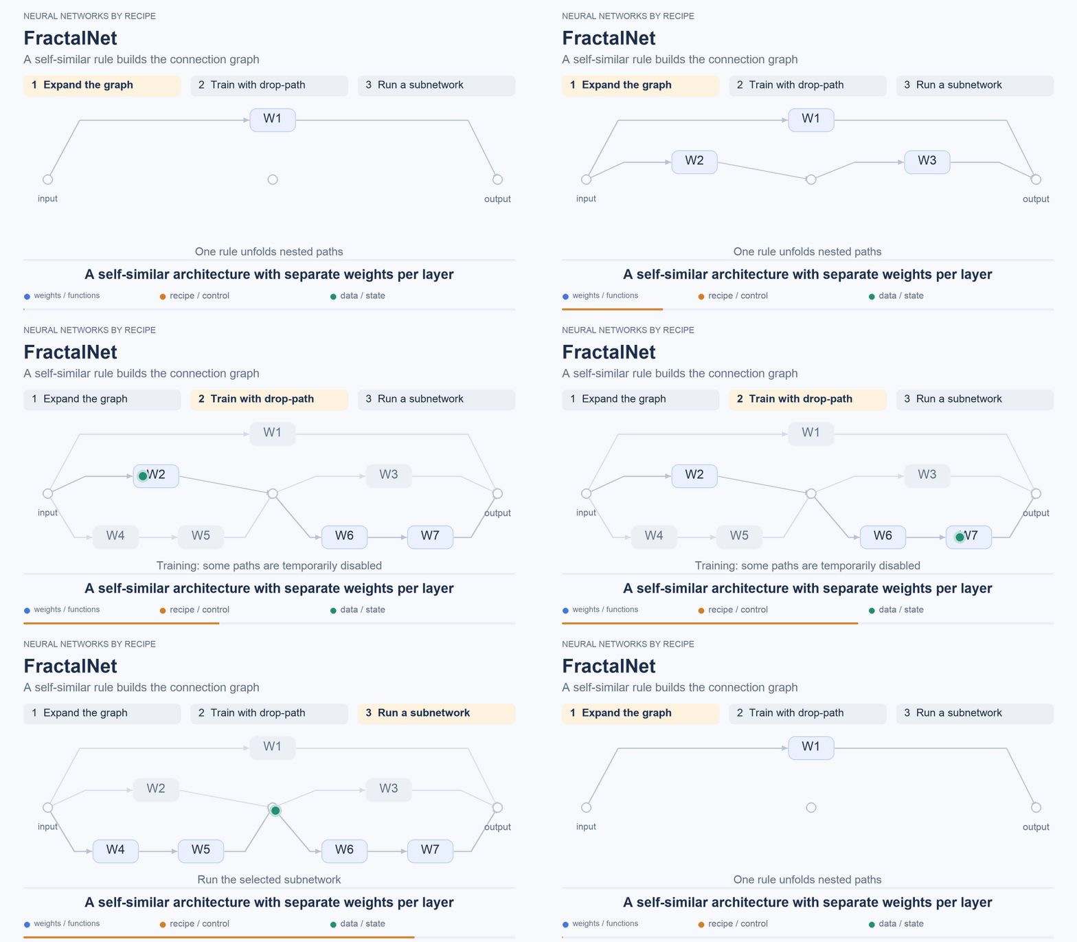
Now let's look at two related fractal approaches. They help distinguish weight generation from the self-similar structure of the network itself. In FractalNet the connection graph of ordinary convolutional layers is made self-similar. The drop-path technique disables individual paths during training so that the network does not rely on just one combination of them. Here, the recipe draws the architecture, while the numerical convolution weights still have to be stored.
These networks classify images on CIFAR, SVHN, and ImageNet. For example, on ImageNet, FractalNet-34 has a top-1 error of 24.12% versus 24.19% for the ResNet-34 C used for comparison. This is the fraction of images for which the first selected class was wrong; the comparison uses validation with ten crops of each image, or 10-crop. Table 2 Shorter subnetworks that can be extracted from the full graph also work.
budgets
Storage — the file size is not reported; a separate 20-layer version in Table 1 has 38.6 million ordinary weights.
Memory — the peak is not reported; the weights and activations of the selected paths are needed.
Time — this depends on the selected path: the authors show a speed–accuracy trade-off between short and long subnetworks. This executes a smaller part of the graph; it does not reconstruct all the weights from a single fractal formula. §3, §4
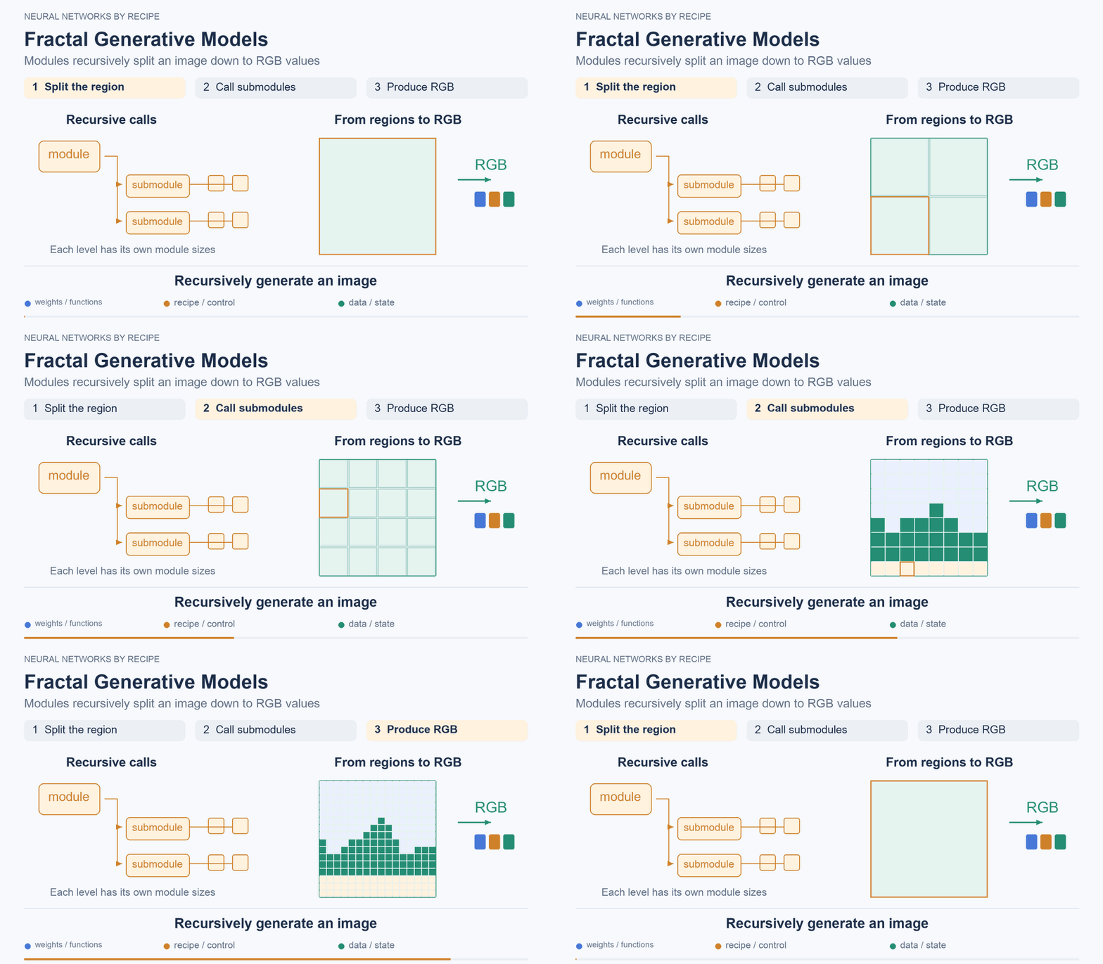
In Fractal Generative Models it is the structure of a generative model that is made self-similar: modules are called recursively, dividing an image into ever smaller parts down to RGB values. Here, “generative” means that the network generates data, rather than the weights of another network. The levels of the model differ in width and depth; this example does not describe the entire network with one shared set of parameters.
On ImageNet 256×256, FractalMAR-H achieves an FID of 6.15, a metric of how close the distributions of generated and real images are, where lower is better. Table 4
budgets
Storage — FractalMAR-H has 848 million parameters; the file size is not reported.
Memory — the overall peak is not reported for this comparison.
Time — with batch 1024 on an H100 PCIe, the authors obtain an average of 1.29 seconds per image. This is not the latency of a single image at batch 1. Table 4, §4.2, §5.2
Recursion over depth: one block, many passes
What if we execute the same block with shared weights many times? Its weights can then be stored once and used repeatedly. Formally, it looks like this:

where  is the intermediate state. The state changes on each pass, while the parameters remain shared. This gives us another way to save resources, though we still have not turned an arbitrary matrix into a fractal formula.
Huginn is a language model: 3.5 billion parameters, trained on 800 billion tokens. Repeating the shared block does not add independent sets of weights, but different passes need intermediate states and a KV cache. The authors separately investigate a bounded cache that overwrites earlier steps.
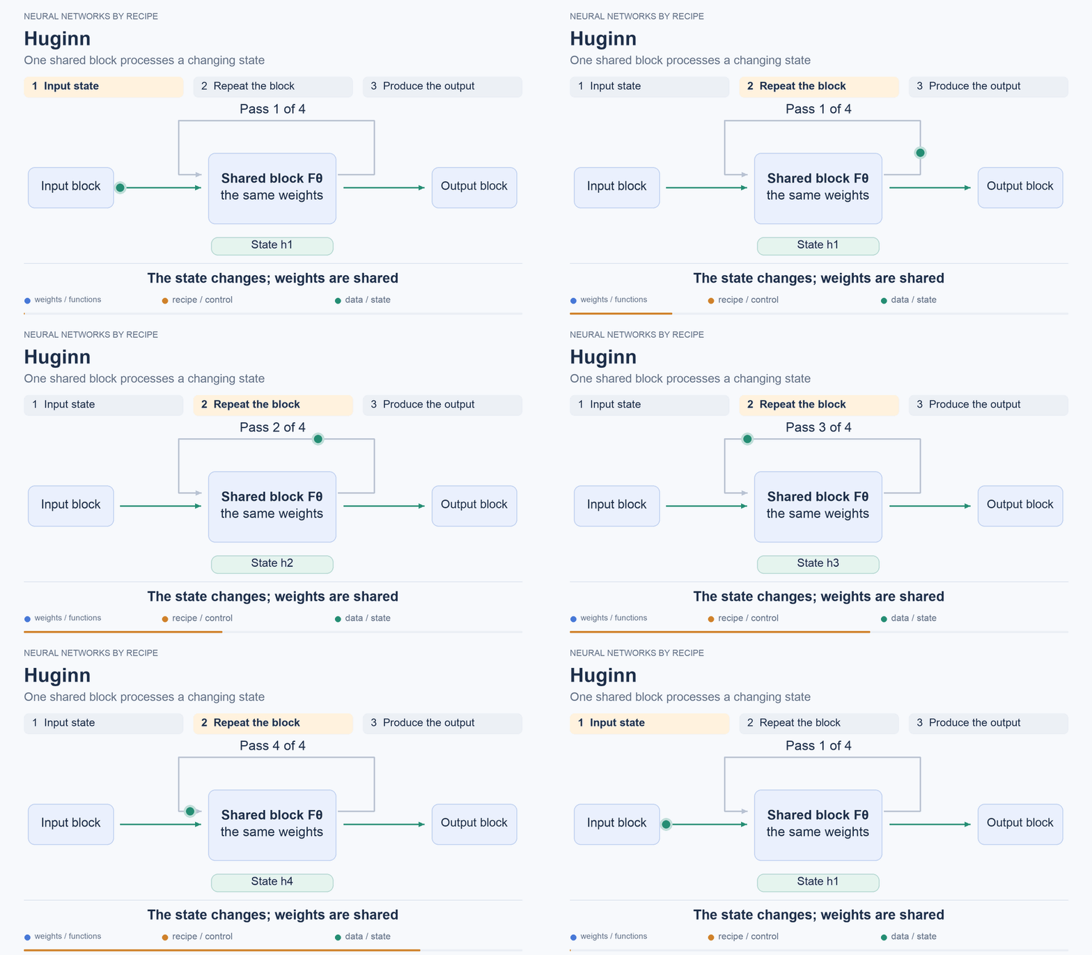
Additional passes through the shared block improve a number of reasoning tasks until the effect plateaus.
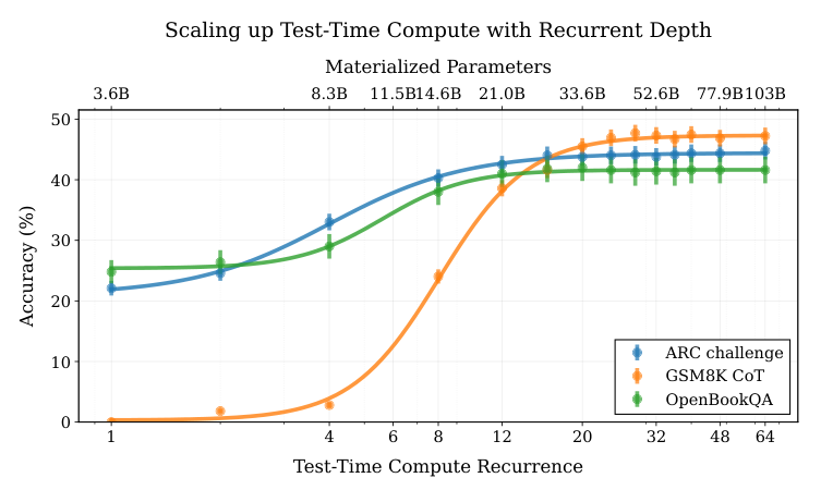
Original Figure 1 from Recurrent Depth: the effect of repetition depends on the task and plateaus. The upper scale, materialized parameters, characterizes the unrolled computation, rather than the size of the stored model. p. 1
budgets
Storage — the file size is not reported;  GB is only an estimate of the space taken by parameters in a 16-bit representation.
Memory — the overall peak VRAM is not reported; the bounded cache reduces the portion of memory use associated with KV.
Time — computing the shared block several times costs more than computing it once; there is no numerical latency comparison here. §6.2
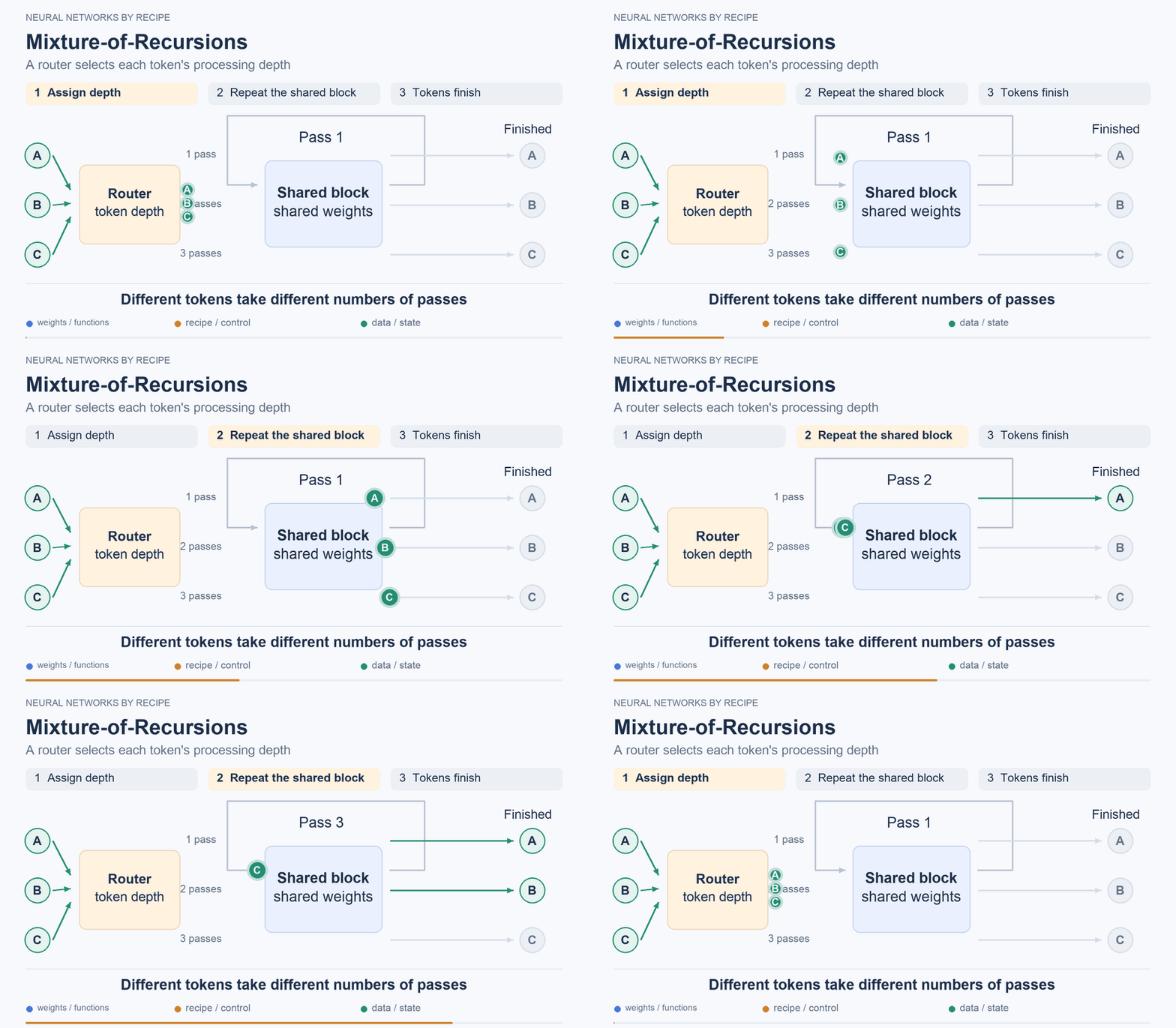
In Mixture-of-Recursions the authors go further: let the model decide how many passes each token needs. A router chooses the depth, while the KV cache management system does not retain an identical set of entries for every possible step. Shared layers reduce the number of independent weights; the selected caching strategy allows more requests to be served at once.
The approach is tested on language transformers built on configurations ranging from 135 million to 1.7 billion parameters. In an additional comparison at the 1.7B scale, with equal training compute budgets, the ordinary model achieves an average accuracy of 48.9% across six tasks, while MoR with two passes achieves 48.4%. The tasks were evaluated in a few-shot setting, with several examples in the prompt. MoR, however, was trained on 26 billion tokens versus 20 billion for the ordinary model. This is a separate quality comparison; the speed measurement below uses a smaller configuration. Table 7
budgets
Storage — the file size is not reported; there are fewer independent weights thanks to the shared layers.
Memory — the full peak is not reported; the feasible batch size is calculated from the weights and KV cache, without the current hidden states.
Time — at the 360M scale, MoR-4 achieves up to 2.06× the throughput, the number of tokens per second, on an H100 with batch 51 versus 32 for the corresponding ordinary model with 34 layers. The measurement excludes KV storage and updates. These numbers do not justify promising a response twice as fast for a single user. §3.3, Appendix E
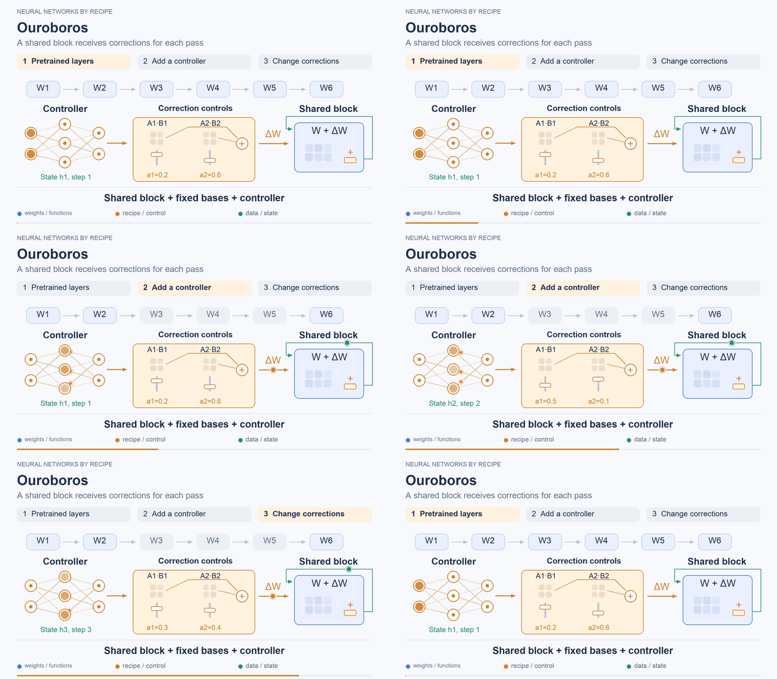
Finally, Ouroboros tries to make an already trained LLM recursive. Some layers are removed, and LoRA corrections are added to the shared block: weight changes specified by a product of small matrices. A controller changes their coefficients depending on the state and pass number. The basis matrices themselves are fixed: they are obtained by an SVD decomposition of the averaged differences between the removed layers and the shared block.
In the main Qwen2.5-3B experiment, 17 out of 36 layers are retained. Quality has not quite worked out yet. Training loss, the value of the error function, decreases by 43.4% relative to the reduced model. But on 12 held-out texts that were not part of training, loss is worse than for the same 17-layer baseline: 5.961 versus 5.690. The authors attribute this to frozen output layers that are not accustomed to the changed states of the shared block. This is their hypothesis, rather than an established cause. And the training improvement certainly cannot be called a recovery of the original Qwen's quality.
budgets
Storage — the complete file size is not reported. Do not rush to calculate the recipe's size from the 9.2 million added trainable parameters alone: according to Table 2, it also needs about 1.8 billion parameters in the frozen base and 7.3 million parameters in the SVD bases.
Memory — peak RAM/VRAM is not reported.
Time — inference latency is not reported; repetitions of the block and the controller add computation. §3–4, Table 2
Selected reproductions: what was checked and what we found
So far, we have examined recipes and their authors' results. What happens if we take the available code and look at the three budgets ourselves? For several papers, this was checked on a CPU: a Xeon Gold 6230, 12 logical cores, and about 45 GiB of RAM, without a GPU. The computations used eight threads and FP32. FI-KAN was trained from scratch, Hyper-Compression was checked with the authors' pretrained weights, and for MoR and Huginn we measured execution of pretrained models. Training large LLMs and their benchmark quality were not reproduced in these CPU experiments.
Each experiment compares two variants; comparing speed across different experiments makes no sense. The package size included weights, settings, the required tokenizer, experiment code, and a file pinning dependency versions, a lockfile, but not installed libraries or data. Peak RAM is the maximum RSS of the process, the physical memory it occupies, including libraries and loading. For files, KB, MB, and GB mean thousands, millions, and billions of bytes; for RAM, we use GiB, or  bytes.
Execution time after warm-up and speed are medians of repeated measurements; for FI-KAN, we use the median of five per-seed medians. Batch 10 means ten images per pass. Decode here means generating subsequent tokens with an existing KV cache, without initial input-text processing. Model preparation time is reported separately where it was measured; those are separate measurements rather than medians of warmed-up passes.
FI-KAN. We repeated a small experiment: KAN and hybrid FI-KAN, four functions, five initial random-number generator values, or seeds, for 500 epochs each. Three rows came out close to Table 3. On the sawtooth function, the hybrid still wins, but the mean error is 0.00127 rather than the published 0.00181. The reproduction is therefore partial. There is also a peculiarity in the authors' protocol: the best epoch was selected by test MSE, the mean squared error on test points. This is not separate validation. The budgets refer to the saved weights of the final epoch, which was not necessarily the best one.
budgets
Storage — for the polynomial experiment, the KAN → Hybrid FI-KAN package takes up about 66.4 → 66.2 KB.
Memory — peak RAM is about 0.22 → 0.22 GiB.
Time — one input after warm-up: 1.88 → 6.99 ms.
Hyper-Compression. Here, we first reconstructed all the weights, after which an ordinary MobileNetV3 ran. On all 10 000 CIFAR-10 test images, the original model achieved 74.42% accuracy, and the compressed model 73.91%. This is close to the authors' 74.41% and 73.93%. We could not exactly reproduce the published 3.61× compression; the reason for the discrepancy has not yet been established.
budgets
Storage — weight and settings files: 6.247 → 1.303 MB, about 4.79 times smaller; the complete package with code and lockfile: 6.335 → 1.392 MB, 4.55 times smaller.
Memory — peak RAM: 0.349 → 0.437 GiB.
Time — reconstruction took 1.27 seconds. From script startup to the first batch, including imports and data preparation: 2.94 → 7.06 seconds. Warmed-up batch 10: 22.93 → 22.61 ms; the ranges overlap, so no speedup is evident here.
MoR. We checked a pretrained pair: 32 layers in the ordinary model and 34 unrolled layers in MoR. It differs from the authors' pair used for the speed test. Here, we used one prompt with 128 input and 16 output tokens; benchmark quality was not checked. The authors' loader makes temporary copies when creating shared layers. Lower memory use after loading therefore does not guarantee a lower overall peak.
budgets
Storage — ordinary model package → MoR-4: 728.235 → 295.586 MB.
Memory — steady RSS: 1.835 → 1.141 GiB, while overall peak RAM is 2.315 → 3.324 GiB. The increased peak is associated with the loading implementation that was checked.
Time — warmed-up decode: 12.06 → 11.07 tokens/s.
Huginn. We compared 4 and 16 passes through the shared block with a full cache. The entire model stayed in RAM during execution. At 16 passes, we separately checked a bounded KV cache. The check is short: one prompt, 16 input tokens, and four output tokens; it cannot establish reasoning quality or long-context behavior.
budgets
Storage — at 4 → 16 passes, the package remains the same: 15.648 GB.
Memory — overall peak RAM with a full cache is about 18.03 GiB in both variants. At 16 passes, the bounded KV cache shrank from 136.4 to 40.1 MB, but the overall loading peak remained around 18 GiB.
Time — warmed-up decode at 4 → 16 passes: 1.66 → 0.42 tokens/s.
Let's put these CPU measurements in one table. Its time column shows execution after warm-up; model preparation is described separately above.
Experiment | Package size | Peak RAM, GiB | CPU execution after warm-up |
|---|---|---|---|
KAN → Hybrid FI-KAN, polynomial | ≈66.4 → 66.2 KB | ≈0.22 → 0.22 | One input: 1.88 → 6.99 ms |
MobileNetV3 → Hyper-Compression | 6.335 → 1.392 MB | 0.349 → 0.437 | Batch 10: 22.93 → 22.61 ms |
Ordinary model → MoR-4 | 728.235 → 295.586 MB | 2.315 → 3.324 | Decode: 12.06 → 11.07 tokens/s |
Huginn: 4 → 16 passes, full cache | 15.648 → 15.648 GB | ≈18.03 → 18.03 | Decode: 1.66 → 0.42 tokens/s |
PocketLLM — our adaptation of the approach. We tried putting this recipe together on a MacBook. Here, we tested the principle itself, rather than reproducing the authors' implementation and results. Instead of Llama or Qwen, we used a pretrained GPT-2 with 124.4 million parameters; computation ran on Metal, on an Apple M2 Pro with 32 GiB of unified memory. All 48 linear attention and FFN matrices, 68.3% of the model's parameters, were replaced with indices, a codebook, and a trained neural decoder. The remaining weights were kept in FP16 and also included in the package size. All matrices were reconstructed before execution.
Predictive quality dropped after compression. We tried recovering it with a short LoRA fine-tuning run: 64 steps on a separate training subset, selecting the saved version by validation. To avoid attributing the ordinary effect of fine-tuning to compression, we applied the same procedure to the dense model. Both received the same step budget; the best versions were selected using the same validation set.
GPT-2 variant | Complete package, MB | Perplexity on the test subset ↓ |
|---|---|---|
Original FP16 | 253.8 | 39.90 |
After compression | 127.0 | 49.83 |
Compression + short fine-tuning | 131.7 | 37.40 |
Dense model + the same fine-tuning | 258.5 | 38.21 |
In our test, the compressed model even achieved lower perplexity after fine-tuning. But this is one seed and 8 192 tokens from the test portion of WikiText-2, rather than a full benchmark; such an experiment does not prove a general quality improvement from compression. A separate load confirmed that the package no longer needs the original dense weights. We ended up with a working storage recipe for a small LLM that still needs space for all the reconstructed weights during execution.
In the following measurements, we compare the original GPT-2 in FP16 without fine-tuning against the compressed model after short LoRA fine-tuning. The LoRA matrices are stored separately in the package, but during loading, the correction is merged once into the reconstructed FP16 weights; there are no additional LoRA operations during decode.
budgets
Storage — original FP16 → compressed after fine-tuning: 253.8 → 131.7 MB, nearly half the size of the original FP16.
Memory — Metal tensors take up about 261.5 MB in both variants; the process's steady RSS increased from about 0.51 to 0.79 GiB. These counters overlap and cannot be added together.
Time — loading until the model is ready: 0.67 → 4.35 seconds, excluding library imports and the first pass. The median for 32 decode steps: 0.351 → 0.436 seconds; the ranges across seven repeats are 0.340–0.393 and 0.349–0.477 seconds, respectively. A repeated independent load of the same compressed package gave 0.407 seconds. Decode was measured with an initial context of 128 tokens: two warm-up repeats and seven more for measurement, with Metal synchronization. In our measurements, the compressed model had a higher median decode time; the ranges of individual repeats overlap.
This is why we needed three budgets: a smaller recipe does not yet mean lower memory use or a faster response. The CPU experiment numbers refer to specific implementations on one server, with the file cache left uncleared and no control over other workloads. For the other papers, we do not yet have enough hands-on evidence; the absence of a measurement does not mean a bad result.
How close are we to an LLM on a low-powered device?
So, in some cases, the drawing of the key really does work. We can store weights as a recipe, reconstruct blocks directly within computation, and use one set of parameters multiple times. But, as you have already noticed, similar words conceal quite different achievements: kilobytes for small networks, fractal functions for approximation, many local codes for LLMs, spectral coefficients and simple factors, and shared layers for repeated passes.
But, as we can see from the approaches discussed, the “kettle” is still a long way off. The papers reviewed do not yet offer a technology that would allow complex neural networks in general, and LLMs in particular, to run on a low-powered device. Optimizing the size of the “cold” model is not enough; something also needs to be done about memory and computational complexity. Even if we are willing to wait a long time for a computation's result, intermediate data has to be stored somewhere or recomputed, which, in my view, currently imposes the more serious constraints.
I think this direction remains just as interesting despite the somewhat gloomy assessment above. Many lines of work bring us closer to the desired outcome of “pocket AI,” and sooner or later this goal will be achieved.